16.6. Slow bulbs

PTC behavior of filament made visible

Author:	Wouter Spaan
Time:	10 - 20 minutes
Age group:	12 - 18
Concepts:	Electricity, PTC, series circuit, IR, FLIR

Introduction

This surprising demonstration makes the PTC (Positive Temperature Coefficient) behavior of light bulbs visible. Explaining the observations requires a lot of thinking-back-and-forth. The demonstration can be inspire students at various levels. It is especially suitable for checking students’ understanding of resistance, current and voltage in series circuits.

Equipment

• Power source

• 4 or 5 identical light bulbs including connection materials.

• optional FLIR camera

Preparation

Set up and already connect the links between the light bulbs, showing clearly that the light bulbs are in series. Draw the circuit on the board.

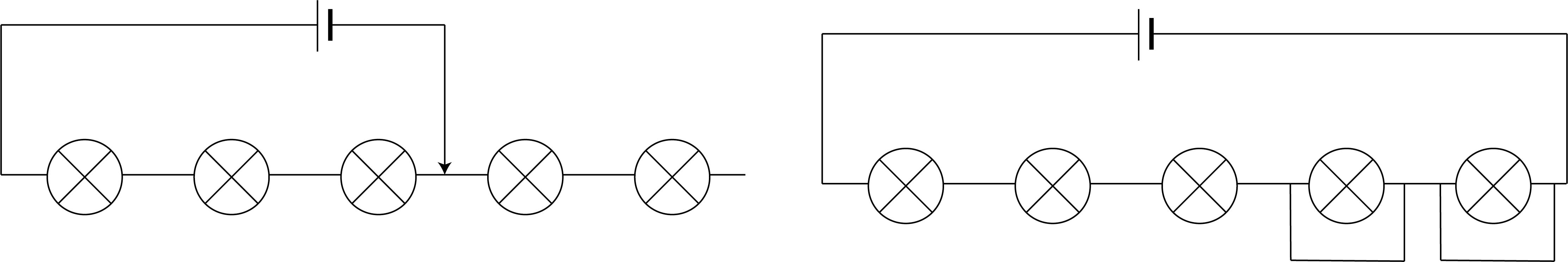
Fig. 16.15 During the demonstration, you continuously move the connection of the negative terminal from left to right, so that the first time only one bulb is switched on and the last time all bulbs are connected. An alternative approach is shown at the right.

Tip

As in the movie, you can short circuit parts of the circuit. The short wired lamp will not light.

Procedure

To start, perform the demo by step-by-step connecting more light bulbs to the power source, with the voltage remaining constant. The students record their observations. Then briefly summarize the observations. Possible observations include:

• Only bulbs between the connections light up.

• The more bulbs are connected, the less brightly they glow.

• The last bulb you connect gradually glows brighter, while the other connected bulbs immediately glow at their final brightness.

• As you connect more bulbs, it takes increasingly longer for the last connected bulb to reach its final brightness.

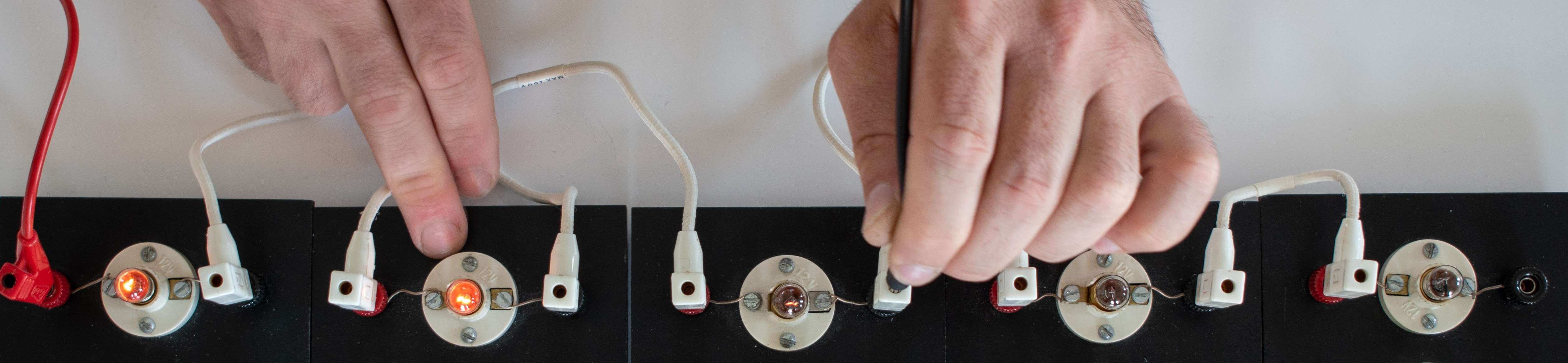
Fig. 16.16 The situation just after moving the connection. The third bulb is barely visible and needs some time to become as bright as the other two.

Then, start a discussion about possible explanations of what was observed. The third and fourth observations are the most interesting; you can use the explanation for the first two to verify students’ prior knowledge. Explaining all these observations requires thinking-back-and-forth, and it is important to pose probing questions and let students use scientific language.

Tip

For explaining the third observation is to ask about what happens to the resistance of a light bulb when the bulb lights up. If the fourth observation hasn’t been made yet, it offers an opportunity for a prediction. Students can also predict what happens to the current during the slow brightening of the last connected bulb. It will decrease; visible with a current meter.

Physics background

The explanation is best linked to the third and fourth observations in the situation of Figure 16.16 where the third light bulb has just been connected: the temperature of bulb 1 and 2 is higher than that of bulb 3 because bulbs 1 and 2 have already been lit up and bulb 3 has not. Hence, their resistance is higher than that of bulb 3, and thus bulbs 1 and 2 receive a larger share of the voltage.

After connecting, the temperature (and thus the resistance) of bulb 3 increases, so it receives more and more voltage (and bulbs 1 and 2 receive less, but the decrease in brightness is not visible to the naked eye). The fourth observation: as more bulbs are in series, the total resistance is greater, and thus the current is smaller, causing the temperature of the last bulb to increase more slowly. This leads to a slower increase in voltage across it and thus a slower increase in brightness. Finally, what happens to the current: the resistance of the last connected bulb increases, so the total resistance in the circuit increases and the current decreases.

The following video shows how the temperature changes. You might want to play the video at double speed.

Follow-up

The demonstration is suitable for further investigations, especially when senors (or an oscilloscope) are available. In the picture below one can observe hysteresis when applying a AC signal to a series circuit with an Ohmic resistor and a light bulb. Using the description by Mooldijk [2005], we made a simulation of this below. Click the at the top right corner.

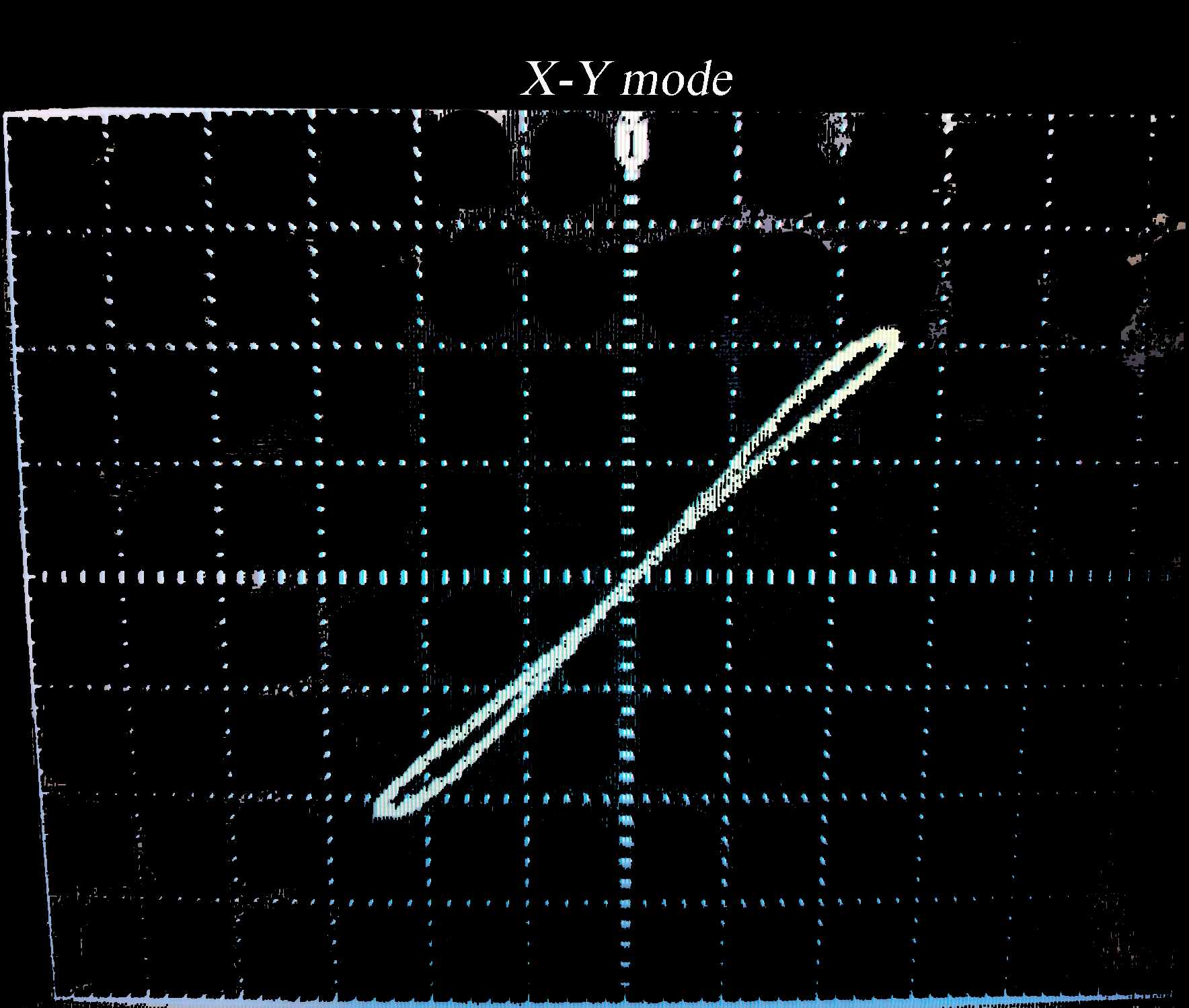
Fig. 16.17 Hysteresis shown with an oscilloscope, signal 1 from the function generator set to 5 Hz, signal 2 from the measurement over the resistor (which is in series with the light bulb). Oscilloscope set to (X-Y)-mode.

import numpy as np
import matplotlib.pyplot as plt
from ipywidgets import interact, FloatSlider

# Model made by Ad Mooldijk

# Constants
U0 = 8          # V
Tg0 = 293      # K
l = 0.0143      # m
d = 0.132e-4    # m
pi = np.pi
A = pi * (d / 2)**2  # m^2
S = l * 2 * pi * (d / 2)  # m^2
Seff = S          # m^2
rho0 = 5.5e-8     # Ohm m
c = 0.13e3        # J/kg/K
rhod = 19.3e3     # kg/m^3
m = rhod * l * A  # kg
ssigma = 5.67e-8  # W/m^2/K^4
alpha = 4.9e-3    # K^-1
dt = float(1e-5)        # s

# Function to run simulation
def run_simulation(f):
    R = rho0 * l / A  # Initial resistance
    Tg = Tg0          # Initial temperature
    t = 0             # Initial time
    times = []
    temperatures = []
    U_x = []
    I_x = []

    # Simulation time parameters
    simulation_time = 3/f  # Total simulation time in seconds
    steps = int(simulation_time / dt)

    for _ in range(steps):
        U = U0 * np.sqrt(2) * np.sin(2 * pi * f * t)
        I = U / R
        Pin = I**2 * R
        Qin = Pin * dt
        dTgin = Qin / (c * m)
        Tg += dTgin
        dPuit = ssigma * Seff * Tg**4
        dQuit = dPuit * dt
        dTguit = -dQuit / (c * m)
        Tg += dTguit
        rho = rho0 * (1 + alpha * (Tg - Tg0))
        R = rho * l / A
        t += dt
        
        # Storing time, temperature, voltage, and current for plotting
        times.append(t)
        temperatures.append(Tg)
        U_x.append(U)
        I_x.append(I)

    # Plotting the results with subplots
    fig, ax = plt.subplots(2, 2, figsize=(12, 6))
    
    # Temperature over time
    ax[0,0].plot(times[int(steps/3):], temperatures[int(steps/3):])
    ax[0,0].set_xlabel('Time (s)')
    ax[0,0].set_ylabel('Temperature (K)')
    ax[0,0].grid(True)
    
    # Voltage vs. Current
    ax[0,1].plot(I_x[int(steps/3):], U_x[int(steps/3):])
    ax[0,1].set_xlabel('Current (A)')
    ax[0,1].set_ylabel('Voltage (V)')
    ax[0,1].grid(True)
    
    ax[1,0].plot(times[int(steps/3):], U_x[int(steps/3):])
    ax[1,0].set_xlabel('Time (s)')
    ax[1,0].set_ylabel('Voltage (V)')
    ax[1,0].grid(True)
    
    plt.tight_layout()
    plt.show()

# Slider for frequency
interact(run_simulation, f=FloatSlider(value=10, min=1, max=50, step=1, description='f in (Hz)'));