17.17. Up and down the hill

Accelerating along a slope

Author:	Freek Pols
Time:	20-30 minutes
Age group:	16 - 18
Concepts:	Newton's first law; acceleration, IOLab, mechanics

Fig. 17.35 The setup consists of the IOlab and a slope.

Introduction

Students often find interpreting and connecting position, velocity, and acceleration in diagrams challenging. In this demonstration, we create a (\(v,t\)) graph during the motion, making it clear that the cart at the highest point does not have an acceleration of 0 m/s²! We use the type of educational activity called ‘think-pair-share’.

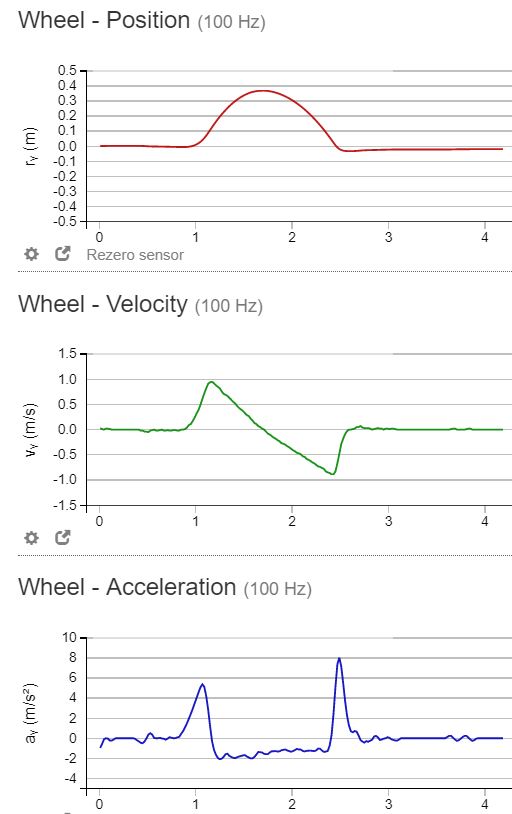
Fig. 17.36 Position, velocity, and acceleration

Equipment

• IOlab

• Slope ~15 cm wide, 50 cm long

• Computer and projection.

Information about using the IOLab can be found here, and an introductory video below (use automated translation):

Preparation

Familiarize yourself with the IOlab, find out hot to read out sensors and start and stop a measurement. Set up the apparatus, distribute graph paper, and connect the IOlab to the computer. Choose the “Wheel 100 Hz” option.

Procedure

1. Explain what will happen in this demonstration. You will give a cart a push, providing it with enough speed to travel up the slope and then roll back down. You will decelerate the cart again so it doesn’t collide. During the movement, you will measure the velocity of the cart and represent it in the (\(v,t\)) graph.

2. What (\(v,t\)) graph will emerge? Ask students to include specific points in the diagram they anticipate (e.g. will the intercept with the y-axis be below, at or above zero? Which point of the graph shows the highest point reached by the cart? Etc.) (think)

3. Ask students to compare their predicted graph with that of their neighbors. (pair)

4. Ask a few students to show and explain their predicted graph. (share)

5. Perform the demo: give the cart a good push up the hill (let go!) and catch it again on the way back down at roughly the same point. Display the (\(v,t\)) graph.

6. Ask students to reflect on the similarities and differences between their predicted graph and the measured graph. Provide, when necessary, the correct interpretation of the measurement results, explicitly link the three graphs ((\(a\),\(t\)); (\(v\),\(t\)); (\(s\),\(t\))) to each other and to the motion of the cart. This way, you can address:

   • At which point in the graph does the cart reach the highest point?

   • What does negative velocity mean?

7. Question to check students’ understanding: A fun children’s game is shooting a ball and then catching it. Draw the (\(v,t\)) graph of the ball from the moment you shoot it until you catch it.

Fig. 17.37 Shooting a ball

Physics background

The kink in the (\(v,t\))-graph at \(v\)=0m/s (see Figure 17.38 occurs because the friction force changes direction at the highest point reached.

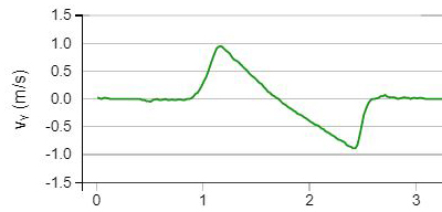
Fig. 17.38 The (\(v,t\))-graph shows a kink at \(v\)=0m/s.

Tip

• Graphically predicting velocity and acceleration is an essential part of this demonstration. Students must realize that the shape they expected may not match the graphs in the measurements, which they may not be able to understand. If such a ‘cognitive conflict’ is followed up appropriately it can result in learning.

• The IOlab can be used in the same way for other motions, such as the transition from uniformly accelerated to uniform motion. Start the car at the top of the slope and let it continue horizontally. Follow the above steps again.

• If you weigh down the IOlab with, for example, 100 g, you will get data with less random error of fluctuations.