15.9. Standing wave with an electric toothbrush#
| Author: | Karel Langendonck |
| Time: | 20-40 minutes |
| Age group: | 17 - 18 |
| Concepts: | Frequency, standing waves |
Introduction#
When a vibration is applied to the end of a taut cord, under certain conditions, a standing wave can arise in the cord. The frequency of the vibration, the wave speed of the resulting wave in the cord, and the length of the cord must be in the correct proportions to each other. In the standard classroom experiment, the frequency is usually varied. But what if the frequency is kept constant and the wave speed and the length of the cord are taken as variables? We use an electric toothbrush as the vibration source.
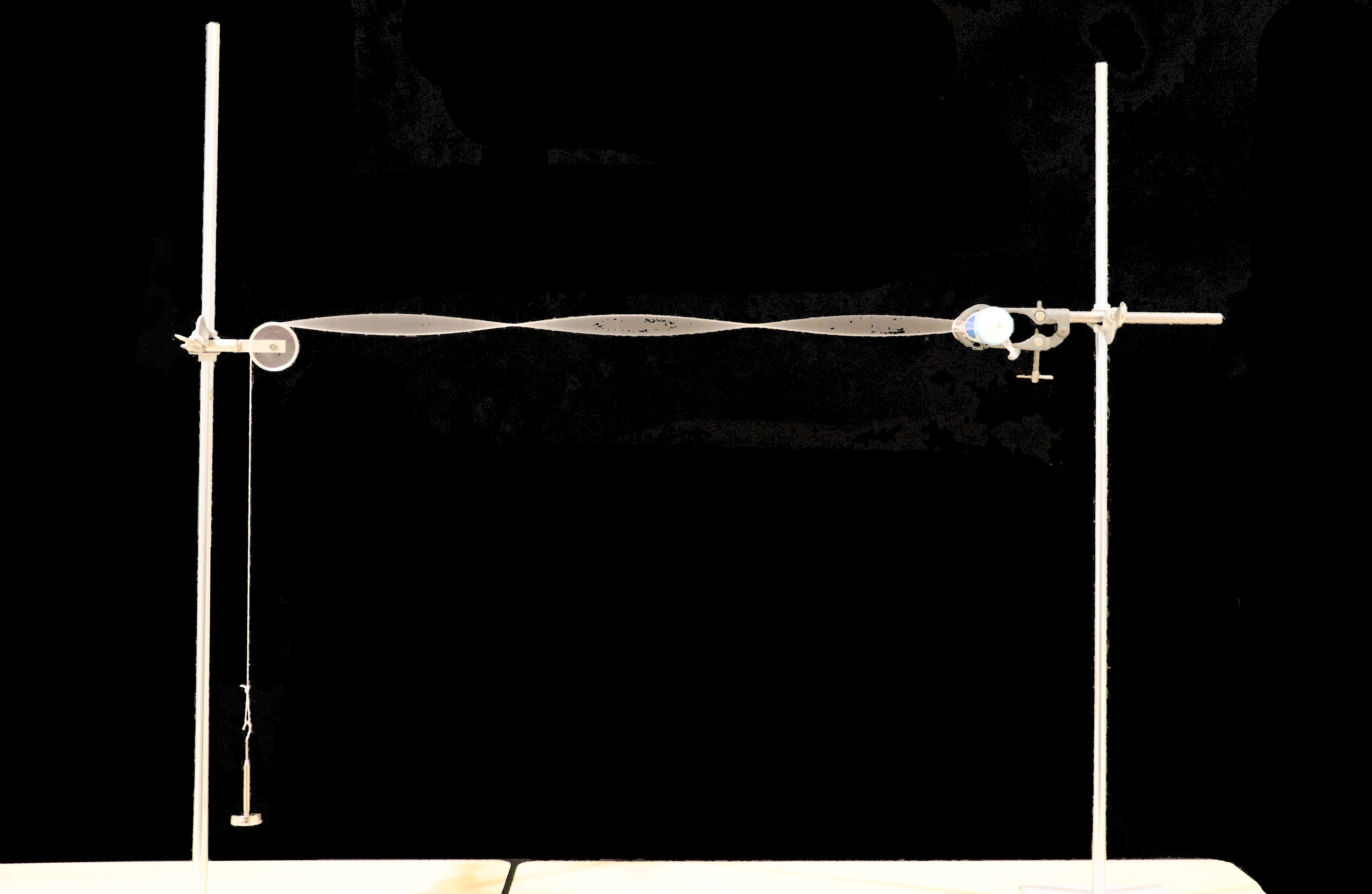
Fig. 15.24 The setup with the toothbrush as frequency generator.#
Equipment#
Electric toothbrush
Cord or elastic band
Pulley
Mass blocks
Tape measure
Accurate scales
Tripod materials
Preparation#
Construct the setup as shown in Figure 15.24. An electric toothbrush is clamped in a tripod, and an elastic band is attached to it. The other end is passed over a pulley, and one or more mass blocks are attached to it.
Adjust the length of the elastic band to get a good standing wave.
Determine the linear mass density of the elastic band.
Procedure#
Let students count the number of half wavelengths visible in the elastic band and then calculate the wavelength using the length of the cord.
Adjust the tension in the elastic band by attaching more (or fewer) weights to the end. Then test again with the length of the elastic band so that a visible standing wave forms again. Have the students determine the wavelength again.
Repeat the previous step several times until, for example, five measurements (of wavelength and mass) are available. You can use the code-cell at the bottom of this page to insert your measurement and make the graph (and do the full analysis). Click the to start the Python script in the code-cell.
Have students draw a graph with wavelength plotted against tension in the elastic. Students will see that there is no proportional relationship. Ask them Which quantities should be plotted against each other to get a proportional relationship?
Then have students draw a graph with the square of the wavelength plotted against tension in the elastic. Now there is a proportional relationship.
Calculate the linear mass density of the elastic band. Or provide it.
Determine the frequency of the electric toothbrush from the slope of the obtained proportional relationship.
Check for understanding with the question: Sketch the (λ², F) diagram that corresponds to an elastic band with a larger linear mass density.
Physics background#
For standing waves, the following formula applies: \(v=\lambda f\)
Here \(v\) represents the wave speed (in m/s), \(\lambda\) represents the wavelength (in m), and \(f\) represents the frequency (in Hz). The wave speed in a taut cord can also be calculated using the following formula: \(v=\sqrt{\frac{F_s}{\rho_L}}\)
In this formula, \(v\) again represents the wave speed (in m/s), \(F_s\) represents the tension in the cord (in N), and \(\rho_L\) represents the linear mass density of the cord (in kg/m). The linear mass density can be determined by dividing the mass of the cord by its length. Both formulas can be equated. This results in: \(\sqrt{\frac{F_s}{\rho_L}}=\lambda f\)
The variables in the experiment are the wavelength and the tension in the cord. By relating these two quantities to each other within this experiment, we can express the above relationship as follows: \(\lambda^2=\frac{F_s}{\rho_L f^2}\)
By plotting the square of the wavelength against the tension in the cord in a diagram, a proportional relationship arises. The slope of the graph is equal to \(\frac{1}{\rho_L f^2}\) and from this, you can then calculate the frequency. An example of a graph is shown in Figure 15.25.
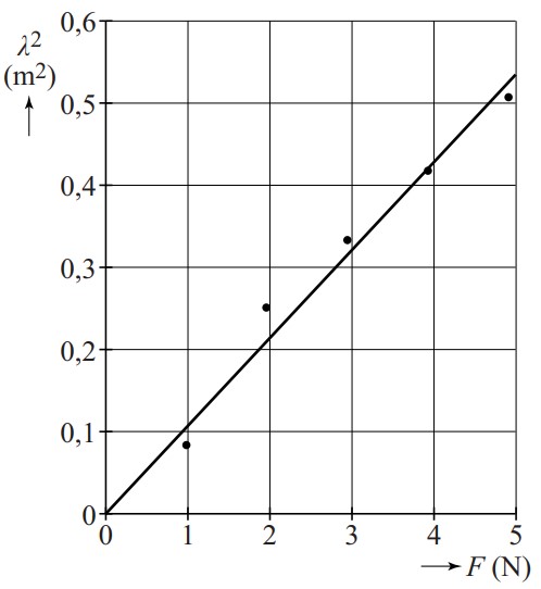
Fig. 15.25 The square of the wavelength plotted against the tension in the cord.#
Tip
The execution of the experiment requires some skill, for which good preparation is necessary. Make sure you have a set of measurement results ready in case obtaining the standing wave in a certain situation does not run smoothly.
The best results of the standing wave occur when the setup is on a stable surface, such as a demonstration table.
Searching for a proportional relationship is a method common in physics. However, for students, this is not easy. Let them first experience that directly plotting the variables against each other does not result in a proportional relationship. This clarifies the relevance of the coordinate transformation. Let the students first think about the necessary coordinate transformation themselves.
It is important for the students to actively follow the experiment and process the obtained measurement results themselves. This way, a certain level of skill is developed. Processing measurement results, drawing graphs, and arriving at a set of data for a proportional relationship are then the learning objectives.
This context has been used in a national Dutch physics exam.
Follow-up#
Using a different elastic band (with a different linear mass density) or a different model or brand of electric toothbrush can inspire further research.
# importing the required libraries
import numpy as np
import matplotlib.pyplot as plt
from scipy.optimize import curve_fit

# insert your measurements
mass = np.array([..,..,..,..,..]) # mass of the objects
wavelength = np.array([..,..,..,..,..]) # wavelength determined

# plotting the measurements
plt.figure
plt.plot(mass, wavelength, 'o')
plt.xlabel('mass')
plt.ylabel('wavelength')

# setting the axis bounds
plt.xlim(0,1.1*max(mass))
plt.ylim(0,1.1*max(wavelength))
plt.grid()
plt.show()
# fitting the data
def function(mass,a):
    return a*np.sqrt(mass*9.81)

var, cov = curve_fit(function, mass, wavelength)

print('The value of a is:', var[0])

# plotting the data and the fit
m_test = np.linspace(0.9*min(mass), 1.1*max(mass), 100)
w_test = function(m_test, var[0])

plt.figure
plt.plot(mass, wavelength, 'o')
plt.plot(m_test, w_test,'r--')
plt.xlabel('mass')
plt.ylabel('wavelength')

plt.xlim(0,1.1*max(mass))
plt.ylim(0,1.1*max(wavelength))
plt.grid()
plt.show()