14.4. Boyle’s law#
How do you verify a physical law?
| Author: | Norbert van Veen and Ed van den Berg |
| Time: | 10-20 minutes |
| Age group: | 14+ |
| Concepts: | Boyle's Law, volume, pressure |
| Skills: | Designing experiment setup, identifying deviations, adjusting model |
Introduction#
Experimentally verifying a formula might seem trivial, but when you ask students in a concrete case - such as Boyle’s Law - how to do it, problems arise. What do you want to measure? How do you measure it? When do you consider results to sufficiently match theory? With Boyle’s law, results often don’t align. Where does it go wrong? This demonstration lets students consider what goes wrong and how to adapt the model to compensate for incorrect assumptions.
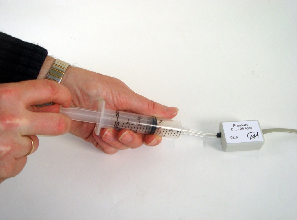
Fig. 14.9 The experimental setup, with a syringe and a pressure sensor.#
Equipment#
Setup with a syringe
A pressure sensor
Measurement software (here we use Coach7)
Preparation#
Set up the apparatus as shown in Figure 14.9. Connect the pressure sensor to an interface and start the measurement program. Record both volume and pressure (at least eight different readings).
Tip
Below we have our measurements, you can run the code cell (and insert your measurements) by clicking above on the .
Especially take measurements at smaller volumes (higher pressures) since this is where issues with residual volume manifest.
Procedure#
Draw a closed volume of gas on the board (circle or square). What happens to the pressure if we decrease the volume? Students will likely have little trouble with this question.
But how does it work exactly? Can we capture this process in some sort of formula? Boyle posited \(p \cdot V = \text{constant}\), or for two situations: \(p_1 \cdot V_1 = p_2 \cdot V_2\). What do you need to do to see if such a theoretical formula aligns with reality? How could you do that? (very brief student discussion in pairs).
Now the teacher shows the setup with a syringe with volume indication and a pressure sensor. What should I do now to verify Boyle’s Law? Let students think for a moment and ask what they came up with.
After a short discussion you collectively arrive at something like: set different volumes and measure the pressure to see if it matches the formula.
Perform the measurements.
import numpy as np
import matplotlib.pyplot as plt
from scipy.optimize import curve_fit

V = np.array([16.0, 14.0, 12.0, 10.0, 9.0, 8.0, 7.0, 6.0, 5.0, 4.0, 3.0])
p = np.array([59.7, 68.3, 79.7, 95.9, 108.1, 119.8, 136.2, 154.9, 186.5, 222.4, 275.1])
How would we know whether our results have verified Boyle’s law?
# calculate p*V, which should be constant according to Boyle's law
print(p*V)
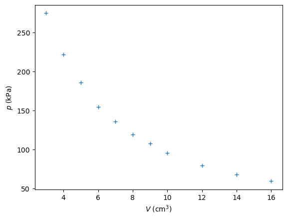
The product \(p\cdot V\) is not constant, let’s explore further and take a look at the graph:
plt.figure()
plt.plot(V, p, '+')
plt.xlabel('$V$ (cm$^3$)')
plt.ylabel('$p$ (kPa)')
plt.show()

# Fit a linear function to the data
def fitfunction(V,a):
    return a*V

val, cov = curve_fit(fitfunction, V, 1/p)

x_test = np.linspace(0, 1.1*max(V),1000)
y_test = fitfunction(x_test, val)

# Plot the data and the fit
plt.figure()
plt.plot(V, 1/p, '+',label='measurements')
plt.plot(x_test, y_test,'r--',label='fit')

plt.xlabel('$V$ (cm$^3$)')
plt.ylabel('$1/p$ (kPa$^{-1}$)')
plt.legend
plt.grid()
plt.show()
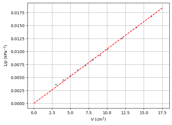
Although there seems to be an inverse proportional relationship, the fitline clearly tells us that something is going wrong…
The measured result don’t match, what could be the reason? (brief student discussion in pairs).
How can we adjust our model \(p \cdot V = \text{constant}\)? Is that justifiable in terms of physics? (add constant term to \(V\), the residual volume).
How can we determine its size? Is there a clever way to transform our graph and extract it from there? (from the deviation of the graph).
Show again the graph of \(\frac{1}{p}\) against \(V\). Ask the students whether it goes through the origin. Have them read the residual volume from the graph.
Another way to find the residual volume is to adapt our model a bit: \(p_1 \cdot (V_1+\Delta V)=constant.\)
# Fit a linear function to the data
def fitfunction2(V,a,dV):
    return a*(V+dV)

val2, cov2 = curve_fit(fitfunction2, V, 1/p)

x_test2 = np.linspace(0, 1.1*max(V),1000)
y_test2 = fitfunction2(x_test2, *val2)

# Plot the data and the fit
plt.figure()
plt.plot(V, 1/p, '+', label='measurements')
plt.plot(x_test, y_test,'r--', label='First model')
plt.plot(x_test2, y_test2,'b--', label='Extended model')

plt.xlabel('$V$ (cm$^3$)')
plt.ylabel('$1/p$ (kPa$^{-1}$)')
plt.legend
plt.grid()
plt.show()
Discuss whether this model corresponds to the data.
Tip
Clearly show the values of the pressure sensor on the digital board.
Show the students that the syringe is being depressed and explicitly mention the volume of the syringe.
Note
There is a more advanced method to compare the correctness of the fit, that is with an analysis of the residuals (data-fit). That method is shown (but hided) below.
Show code cell source
plt.figure()
plt.plot(V, 1/p-fitfunction(V,*val), 'r+', label='First model')
plt.plot(V, 1/p-fitfunction2(V,*val2), 'b+', label='Extended model')
plt.xlabel('$V$ (cm$^3$)')
plt.ylabel('residuals')
plt.legend()
plt.hlines(0,0,max(V),linestyles='dashed')
plt.show()

plt.figure()
plt.hist(1/p-fitfunction(V,*val), bins=7, color='r', alpha=0.5, label='First model')
plt.hist(1/p-fitfunction2(V,*val2), bins=7, color='b', alpha=0.5, label='Extended model')
plt.vlines(0,0,6)
plt.xlabel('residuals')
plt.ylabel('frequency')
plt.legend()
plt.show()
Physics background#
The pressure and volume of a closed quantity of ideal gas behave according to Boyle’s Law. Due to the residual volume of the hose and the pressure sensor, the hyperbola of the measurements will deviate slightly from the volume that is read from the syringe. If we call the residual volume \(\Delta V\), then Boyle’s Law can be written as:
The ideal gas law assumes that the attraction between molecules is zero and that the molecules themselves are point particles that occupy no volume. Van der Waals took into account the attraction and volume of molecules:
The pressure is corrected for attraction between molecules and also the volume of molecules is taken into account. These corrections become important at a higher density. The constant b is then roughly the volume of 1 mole, and the constant a depends on the attraction between molecules. These constants are determined empirically. For details, we refer to well-known textbooks such as [Young et al., 2014], chapter 17.
We fit our data using this model below.
Show code cell source
# Fit a linear function to the data
def fitfunction3(V,a,dV,b,c):
    return a*(V+dV)+b/(V+dV)+c/(V+dV)**2

val3, cov3 = curve_fit(fitfunction3, V, 1/p)

x_test3 = np.linspace(0.8*min(V), 1.1*max(V),1000)
y_test3 = fitfunction3(x_test3, *val3)

# Plot the data and the fit
plt.figure()
plt.plot(V, 1/p, '+', label='measurements')
plt.plot(x_test3, y_test3,'r--', label='Van der Waals model')

plt.xlabel('$V$ (cm$^3$)')
plt.ylabel('$1/p$ (kPa$^{-1}$)')
plt.legend
plt.grid()
plt.show()
Follow-up#
What influence does a lower or higher temperature have on gas pressure measurements?
The graphical model also shows the Van der Waals gas model. Plot this graph alongside Boyle’s law and ask students to explain how the differences arise. At what pressures does Boyle’s law deviate from Van der Waals’ gas law?
References#
Hugh D Young, Roger A Freedman, and Albert Lewis Ford. University physics with modern physics. Pearson New York, 2014.