15.10. Physics of the panflute#
Determination of the speed of sound
| Author: | Freek Pols |
| Time: | 15-20 minutes |
| Age group: | 16 - 18 |
| Concepts: | Standing waves, sound, frequency |
Introduction#
In this demonstration, we use a homemade panflute and take measurements of the lengths of the tubes and the corresponding frequency using the Phyphox app. The theory of standing waves in an open and closed tube then provides an accurate determination of the speed of sound.
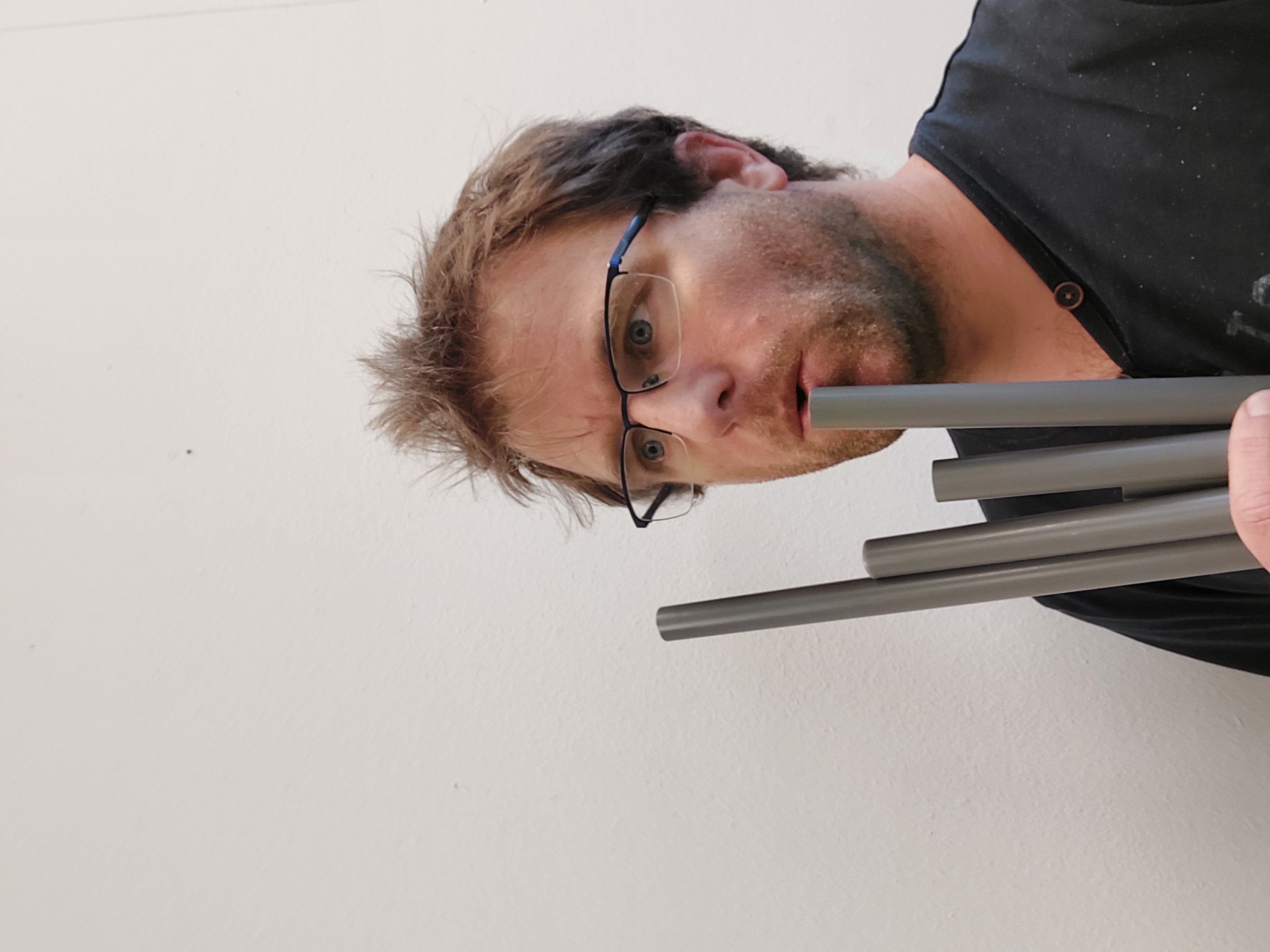
Fig. 15.26 The demonstration requires minimal equipment: a few PVC tubes of different lengths and your phone.#
Equipment#
5 PVC tubes of different lengths but with the same diameter
Phone with Phyphox app
Preparation#
Start the Phyphox app and load the Python in browser tool by clicking the rocket () at the top of this page. You can now use the code-cell at the bottom of this page.
Procedure#
Blow over the top end of a long tube with your thumb on the bottom end of the tube.
Question: Is the pitch higher/lower or equal to the pitch you get when blowing over a short tube? Why?
Blow over the short tube to confirm.
Explain that you want to determine the relationship between the length of the tube and the pitch (resonant frequency). Then measure the corresponding frequencies for all tube lengths using the Phyphox app for frequency measurements.
Record the data in the code-cell at the bottom of this page. You can ask the students to determine the speed of sound themselves, assuming \(L = \frac{\lambda}{4}\). They will then see that the calculated wave speed increases each time. This is strange! You can exploit this experience of ‘strangeness’ to make it plausible that it is useful to analyze the results with the computer/graphically. Then run the code-cells so that you see the graphs.
Question: Is it true that the frequency decreases as the tube length increases?
During the explanation pay attention to the linear relationship between the frequency of the fundamental tone \(f\) and the reciprocal of the tube length \(l\). From the slope coefficient find the speed of sound.
Question: Does the value actually match when using only one measurement? Why not?
Blow hard over the tube. You will clearly hear an overtone that you can measure.
A question to check students’ understanding: Make a sketch showing how the waves of possible overtones can fit in the tube. Calculate the resonant frequency based on that drawing.
Verify this frequency with a measurement.
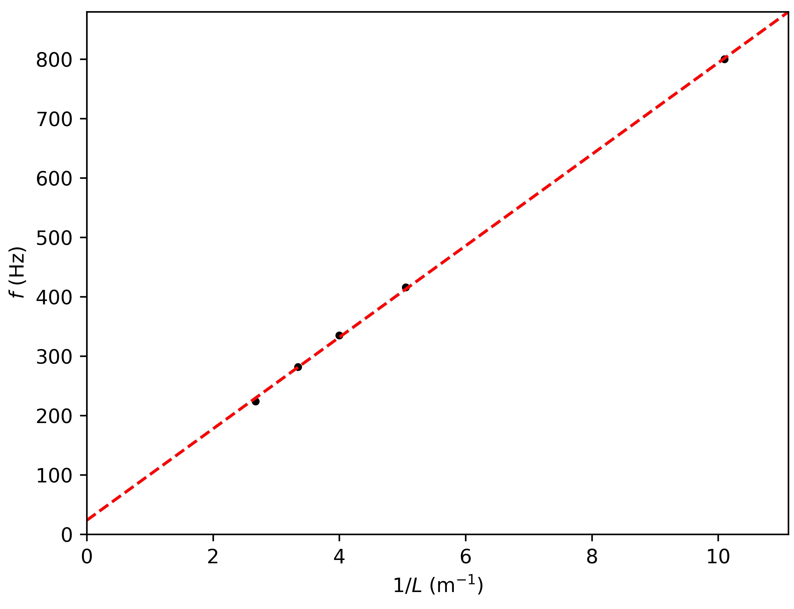
Fig. 15.27 The data presented with coordinate transformation. Based on the function fit, the speed of sound in air is determined.#
Physics background#
In the open-closed tube, the fundamental frequency is equal to: \(f=\frac{v}{\lambda}=\frac{v}{4 l^{\prime}}\)
Here, we note \(l^{\prime}\) because the node does not lie exactly at the opening of the tube but just outside it. So: \(l^{\prime}=l+\Delta l\)
Where \(\Delta l\) is a systematic deviation. It is because of this deviation that you need measurements at multiple lengths.
Tip
When blowing hard on the tube, you clearly hear one of the overtones.
A Dutch national exam question also addresses this demonstration and can be used for further practice.
Instead of using tubes of different lengths, you can also submerge one end in a tall measuring cylinder. The effective length of the tube is then easily adjustable. An interesting variant of this demonstration can be seen here: https://youtu.be/eaeyIJAYsvo.
have described this experiment in The Physics Teacher.
References#
Code-cells#
#Loading libraries
import numpy as np
import matplotlib.pyplot as plt
from scipy.optimize import curve_fit

#Measurements
L = np.array([9.9, 19.8, 25.0, 29.9, 37.3])*1e-2 #input in cm
u_L = np.ones(len(L))*0.001 #m
f_0 = np.array([860, 439, 352, 293, 233]) #Hz
u_f_0 = np.ones(len(f_0))*3 #Hz 5, 2, 1, 3

lambda_f_0 = 4*L
u_lambda_f_0 = 4*u_L
print("Successfully loaded the data")
#Plotting the data
plt.figure()
plt.errorbar(L,f_0,xerr=u_L,yerr=u_f_0,linestyle='none')
plt.plot(L,f_0,'k.')
plt.xlabel('$L$ (m)')
plt.ylabel('$f$ (Hz)')
plt.show()
#functionfit
def funcfit(x,v,dL):
    return v/(x+dL)

var, cov = curve_fit(funcfit,lambda_f_0,f_0,p0=[343,2e-2])
print(var)
print()
print('The velocity of sound in air is:', round(var[0],0),'+/-',round(np.sqrt(cov[0,0]),1),'m/s')
#plotting the data and the fitfunction
x = np.linspace(0.9*min(lambda_f_0),1.1*max(lambda_f_0))
y = funcfit(x,var[0],var[1])

plt.figure()
plt.plot(x,y,'r-')
plt.plot(lambda_f_0,f_0,'k.')
plt.xlabel('$\lambda$ (m)')
plt.ylabel('$f$ (Hz)')
plt.xlim([0.95*min(lambda_f_0),1.05*max(lambda_f_0)])
plt.show()