19.9. Transit of a planet#
Simulating planet transits
| Author: | Norbert van Veen |
| Time: | 10 minutes |
| Age group: | 14 - 18 |
| Concepts: | Transits, planets, observation, exoplanet |
Introduction#
Most students will not be familiar with the transit of an exoplanet, though exoplanets might fascinate them. With a relatively simple setup, you can give your students a glimpse of how such an observation works. The calculations can be extrapolated to real-life scenarios.
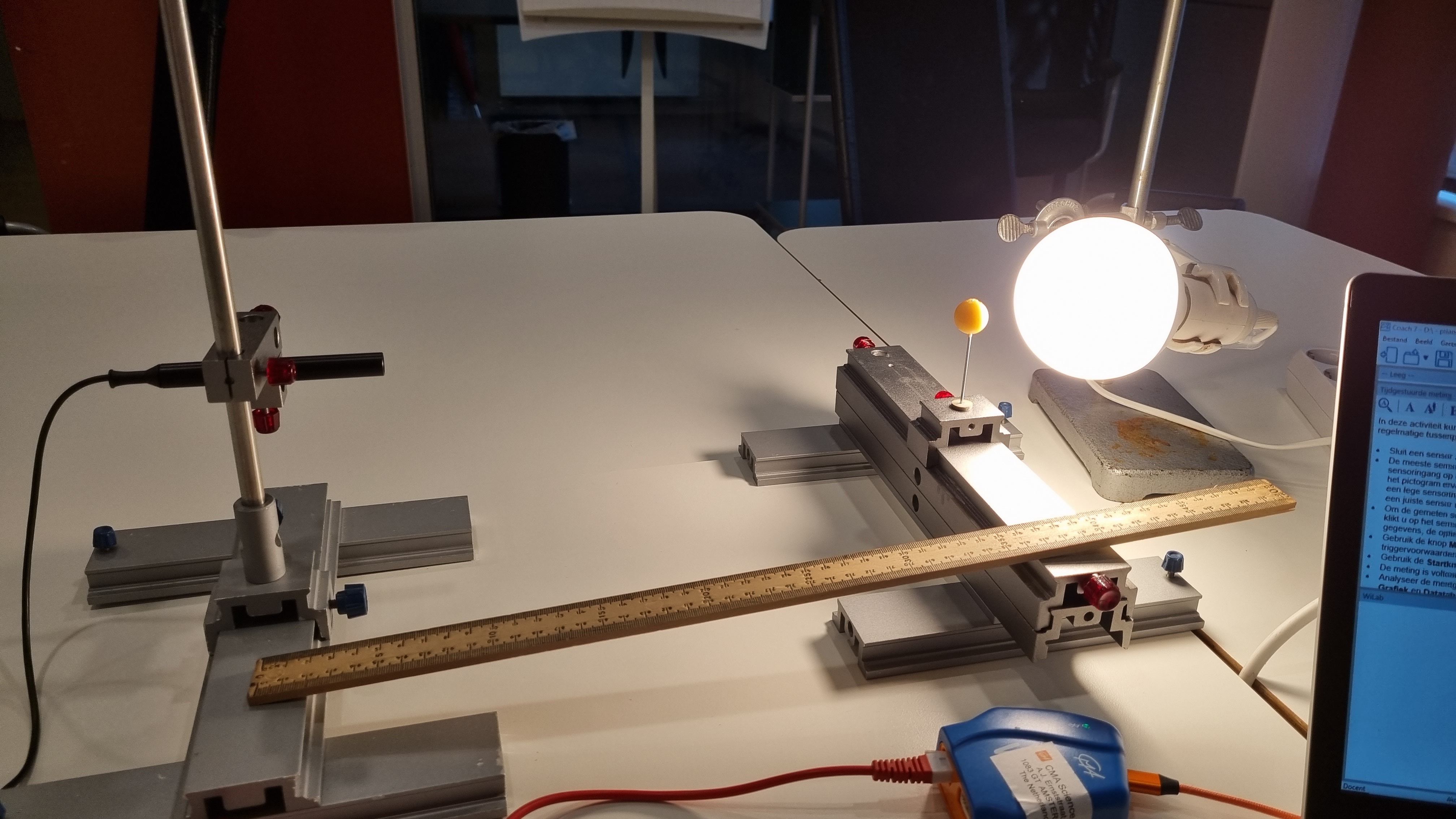
Fig. 19.19 Setup to measure a transit.#
Equipment#
LED lamp (large opaque lamp) in holder
Measuring tape
Caliper
Light sensor
Sphere in a rider of an optical case
Tip
There are great simulations making transits even more clear.
Preparation#
Align the setup so that the light sensor, sphere, and opaque lamp are in line.
Darken the room.
Connect the light sensor to a real-time measurement device or datalogger. Ensure that the amount of light from the lamp does not overpower the light sensor.
Change the distance between the light sensor and the lamp. Use a sphere with a diameter of approximately 1/5 or smaller than the diameter of the lamp.
Display the computer screen via a projector or interactive whiteboard.
Procedure#
Start the measurement. Move the rider with the sphere past the lamp at a constant speed. Stop the measurement.
Enlarge the light dip in the graph by zooming in with the mouse. See Figure 19.20.
How can you determine the duration of the transit?
Ask the students to sketch how the transit curve would look if the planet moved slower/faster.
Ask the students to sketch how the transit curve would look if the planet were larger/smaller.
Provide the formula below and ask the students to apply it to the situation. Provide the diameter of the lamp. Here, \(H\) represents the brightness or intensity of the received light. \(\frac{H_{dip}}{H_{star}} =1-(\frac{r_{planet}}{R_{star}})^2\)
Let students calculate the radius of the planet using the formula.
A question to check students’ understanding: In what way(s) does this demonstration deviate from actual observations of exoplanets?
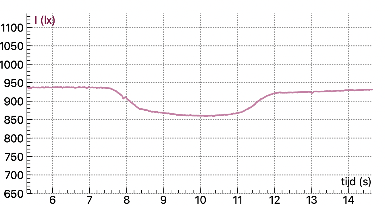
Fig. 19.20 The light dip of the transit, measurements taken using the software Coach.#
Physics background#
In this setup, you simulate a transit of an exoplanet with a sphere in front of an opaque lamp. Unlike a ‘real’ star, the lamp will have a diverging beam of light at the location of the ‘planet’. Also, the proportions are not to scale compared to the ‘real’ situation. Nevertheless, you get a decent dip in light intensity, which can be used to clarify the idea of measuring a transit.
The light sensor used has a spatial measurement angle of 50 degrees and will therefore be able to measure a large part of the light from the opaque lamp at this distance. This explains the relatively large dip you measure.
During a transition, an exoplanet will block a small portion of the light from its star, allowing very advanced equipment to measure a dip in light intensity. The captured starlight is parallel. By measuring multiple consecutive dips, you can derive the orbital period of the planet. Because the mass and luminosity of a star are known, you can derive the orbital radius of the exoplanet using Kepler’s third law, and then the mass, density, and gravitational acceleration. In some cases, you can also determine the composition of gases in the planet’s atmosphere by measuring its absorption spectrum.
Tip
We used an 8 W LED opaque lamp with a diameter of 95 mm. Make sure the LED lamp does not flicker. Check this with the slow-motion camera mode of a phone. Our planet was a sphere with a diameter of 18 mm. We set the light sensor to 1500 Lux.
The setup with the rider also reflects light from the lamp, resulting in a slightly higher zero brightness (\(H_0\)). Try to cover anything that can reflect light. Optionally, slide a PVC pipe over the light sensor to prevent scattered light.