18. Velocity transformation & Doppler effect

18.1. Velocities

Imagine we have two space ships moving each with a speed of \(\frac{3}{4}c\) as shown below. What is the speed that either the red or yellow space ships sees for the other space ship speed?

We should, first of all realize, that the information regarding the velocity of the two space ships is given by an observer \(S\) who is neither in the red nor the yellow ship. We need to transform this information to an observer in the red or in the yellow ship.

Fig. 18.1 Two space ships approaching each other.

For the GT we have derived the transformation to be

\[ v'_{x'} = v_x-V \]

So let’s translate our velocity information from the observer \(S\) to someone in the red ship. The relative velocity between \(S\) and the red ship is \(V=\frac{3}{4}c\). Thus according to the observer in the red ship, \(S_R\), her velocity is \(V'_R = V_R -V_R =0\), obviously.

However, she will denote the velocity of the yellow ship as \(V'_y = V_y - V_R = (-3/4 - 3/4)c = \frac{3}{2}c > c\). In the world of Galilei and Newton, this is no problem at all: velocities can be as big as you can imagine. However, in reality, this is not true. We have to use Special relativity if the velocities start to approach \(c\). It is not possible for any object to move faster than the speed of light, as we will see later.

In the above, we have only looked at the velocity component in the \(x\)-direction. We have in addition found \(v'_{y'}=v_y, v'_{z'}=v_z\).

As our universe does not follow Galilei and Newton, we need to derive the transformation/addition formula for velocities with the LT. So, let’s do it.

Let us start from the definition of velocity (assuming we deal with constant velocities, so we don’t need to worry about differentiation and integration). We will denote velocities by \(u\) to avoid confusion with \(V\), the relative velocity between the two observers.

\[ u'_{x'} = \frac{x'_2-x'_1}{t'_2-t'_1} =\frac{\Delta x'}{\Delta t'} \text{\ and \ } u'_{y'} = \frac{y'_2-y'_1}{t'_2-t'_1} =\frac{\Delta y'}{\Delta t'} \quad (*) \]

We have left out the \(z\)-component as that will be completely analogous to the \(y\)-coordinate.

We need to use the LT to transform \((ct',x',y')\) to \((ct,x,y)\):

\[\begin{split} \begin{array}{rcl} x'_2-x'_1 &=& \gamma \left ( x_2 -\frac{V}{c} ct_2 \right ) -\gamma \left ( x_1 -\frac{V}{c} ct_1 \right )\\ &=& \gamma (x_2-x_1)-\gamma \frac{V}{c}(ct_2-ct_1) \\ \\ y'_2-y'_1 &=& y_2 - y_1 \end{array} \end{split}\]

and

\[\begin{split} \begin{array}{rcl} ct'_2-ct'_1 &=& \gamma \left ( ct_2 -\frac{V}{c} x_2 \right ) -\gamma \left ( ct_1 -\frac{V}{c} x_1 \right )\\ &=& \gamma (ct_2-ct_1)-\gamma \frac{V}{c}(x_2-x_1) \end{array}\end{split}\]

From the last line it is clear that also the \(y,z\) components of the velocity \(\vec{u}\) will be influenced by the transformation although the relative motion between the two observers is only along \(x\). Substituting the expressions for the space and time difference into equation \((*)\), we obtain

\[\begin{split} \begin{array}{rcl} u'_{x}&=& \displaystyle{\frac{\gamma \Delta x - \gamma \frac{V}{c}\Delta ct}{\gamma \Delta ct - \gamma \frac{V}{c}\Delta x} = \frac{\frac{\Delta x}{\Delta t}-V}{1-\frac{V}{c^2}\frac{\Delta x}{\Delta t}}}\\ \\ &=& \displaystyle{\frac{u_x-V}{1-\frac{Vu_x}{c^2}}} \end{array} \end{split}\]

For the transverse components \(y,z\), we obtain due to the change of the time interval

\[ u'_{y'} = \frac{\Delta y}{\gamma \Delta ct - \gamma \frac{V}{c}\Delta x} = \frac{u_y}{\gamma \left (1-\frac{Vu_x}{c^2}\right )} \]

In the limit of \(u_x,V\ll c\) both formulas reduce to the Galileo transformation as required. For \(u_x\to c\) and \(V\to -c\) the combined velocity will stay smaller than \(c\). Check.

The formula for the velocity transformation/addition are not so easy to remember. Later you will see how to derive them from the transformation properties of the 4-velocity, which is much easier to remember. In addition the formula follows also directly from the interpretation of LT as rotations in Minkowski space.

For our example of the two approaching space ships, \(u_x=-\frac{3}{4}c, V=\frac{3}{4}c\) we find for the speed of the yellow approaching the red ship

\[ \frac{-\frac{3}{4}-\frac{3}{4}}{1+\frac{3}{4}\frac{3}{4}}c=-\frac{24}{25}c <c \]

This is again smaller than \(c\). For the other ship we find of course the same, but with different sign.

”Velocity addition with \(\beta\equiv u/c\)”

If we state all velocities (for the 1D case) as \(\beta_1 = \frac{u}{c}\) and \(\beta_2 = -\frac{V}{c}\) than the addition takes on an easy form

\[ \beta = \frac{\beta_1 + \beta_2}{1+\beta_1 \beta_2} \]

18.2. Doppler effect

The Doppler effect is well-known from waves. You will learn the details about this in classes like Introduction to Waves.

You know it from daily life. If a car is passing you at high speed, the frequency of the sound you hear changes from approaching to driving away from you. The received frequency \(f_{obs}\) by you is higher than the emitted frequency \(f_{src}\) while the car is approaching, and smaller when it drives off.

Here we investigate the effect of a moving source that is emitting light with \(f_{src}\) (electro-magnetic waves). This is one of the few cases where the relativistic case is easier than the classical effect. In the latter it matters if the source is moving or the medium. For EM-waves, however, there is no medium (aether) as we have seen which simplifies things.

Fig. 18.2 Effect on sound waves due to motion.

For the case of an observer with speed \(v_{obs}\) and speed of sound in the medium \(u\) and moving source \(v_{src}\) (e.g. a car) the classical formula of the frequency shift is

\[ f_{obs} = f_{src}\frac{u\pm v_{obs}}{u\mp v_{src}} \]

where for the stationary observer & medium, we have \(+/-\) and for the moving observer and stationary source \(-/+\).

The origin of the observed frequency shift of a moving source is visible in the picture. In the direction of motion, more wave maxima arrive per unit time, as the car is moving closer between two wave maxima.

For the relativistic effect we consider a moving source with velocity \(\vec{u}\) with observer \(S'\) relative to \(S\). The frequency of the source is \(f_0=\frac{1}{T_0}\) in the rest frame, with \(T_0\) the period of the oscillation.

Fig. 18.3 Observer S’ and source both moving with respect to S.

We now consider the situation for \(S\) as shown in the figure below. The position of the source \(\vec{r}_0\) is indicated with the star \(*\).

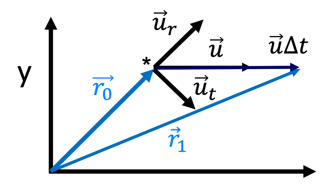
Fig. 18.4 Observer S’ and source both moving with respect to S

We do know that according to \(S'\), the proper frequency is \(f_0\) and the proper period \(T_0 = 1/f_0\). Thus if a maximum is send at \(t'_0\) the next one will be at \(t'_0 + \frac{1}{f_0}\).

\(S\) will denote the first maximum with time \(t_1 = t_0\), but will have to take time dilation into account for the second one: \(t_2 = t_0 + \frac{\gamma}{f_0}\). Note that these two time instants are the moments, according to \(S\) when the two maxima are send, not when they are received by \(S\).

During this time interval \(\frac{\gamma}{f_0}\) the source moves from \(\vec{r}_0\) to \(\vec{r}_1=\vec{r}_0+\vec{u}\frac{\gamma}{f_0}\). Thus, the distance that the second maximum has to travel is different from that of the first one, just like in the classical Doppler case.

We consider the 2 consecutive wave maxima that are emitted in \(S'\) and received in \(S\):

• 1\(^{st}\) maximum in \(S'\) at \(t'_0\), that is received in \(S\) at \(t_1=t_0 +\frac{r_0}{c}\). The additional time \(\frac{r_0}{c}\) is needed for the light to travel from \(\vec{r}_0\) to the observer at the origin of \(S\).

• 2\(^{nd}\) maximum in \(S'\) at \(t'_0+\frac{1}{f_0}\), is received in \(S\) at \(t_2=(t_0+\frac{\gamma}{f_0})+\frac{r_1}{c}\).

To move further we split the velocity of the source into a radial component (in line to the observer in \(S\)) and a tangential part perpendicular \(\vec{u}=\vec{u}_r+\vec{u}_t =u_r \hat{r} +u_t \hat{t}\). If the distance \(r_0 \gg \vec{u} \frac{\gamma}{f_0}\) then the distance \(r_1 = r_0 + u_r \frac{\gamma}{f_0}\).

Note that we could drop the vector notation here from the exact relation above. Classically only the radial component is relevant as only the distance matters.

With this simplification on the distances we can compute \(t_2\)

\[ t_2 = (t_0+\frac{\gamma}{f_0})+\frac{r_1}{c} \approx t_0+\frac{\gamma}{f_0} + \frac{r_0+u_r \frac{\gamma}{f_0}}{c} \]

For the frequency \(f\) in \(S\) we now subtract the two arrival times

\[ \frac{1}{f} =t_2-t_1 = \frac{\gamma}{f_0}+ \frac{u_r}{c}\frac{\gamma}{f_0} \]

Rewriting this into a ratio of the emitted and received frequency, we obtain for the relativistic Doppler effect

\[ \frac{f_0}{f} = \gamma \left (1+\frac{u_r}{c} \right ) = \frac{1+\frac{u_r}{c}}{\sqrt{1-\frac{u^2}{c^2}}} \]

Please observe that the \(\gamma\) factor is of \(\gamma(u)\) that means even for only tangential movement \((u_r=0)\) there is a Doppler shift.

18.2.1. Cosmic background radiation

The most well-known frequency shift is the red-shift from the expanding universe.

The astronomer Edwin Hubble first found in the 1920s that the universe does not only consists out of our own galaxy, the milky way, but there must be (many) other galaxies, which were called nebula at that time. Second he could show that all further away galaxies move away from us by measuring the Doppler shift of well-known emission lines of stars and their distance from periodic intensity variation of Cepheid Variable stars. It turned out that the distance of the galaxies \(d\) was roughly linearly proportional to the red-shift which is again linearly related to the radial velocity \(v\) as we derived. This is known now as Hubble’s law \(v=H_0 d\) with the Hubble constant \(H_0 \sim 70\ km/s/Mpc\)). Further away galaxies move faster away, but why? And why is no galaxy approaching us?

At end of the 1920s Georges Lemaître applied Einstein general theory of relativity to cosmology and found that the universe must be expanding, while it started in a “primeval atom”, now known as the Big Bang. He could explain the red-shift relation from the expanding universe hypothesis.

The Big Bang theory was highly debated early on, in particular by Einstein, but is now fully accepted. The strongest experimental evidence was the discovery of the cosmic background radiation in 1965 (by accident).

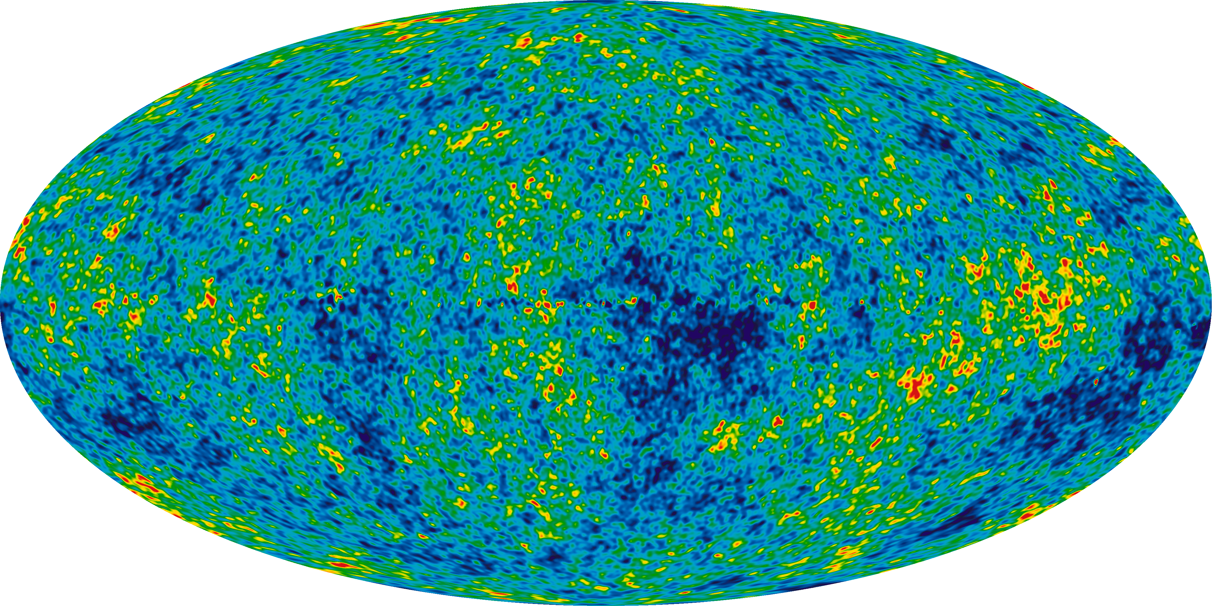
The whole cosmos is nearly uniformly filled by a background radiation of about 2.7 K (wavelength in the \(\mu\)m range) with small inhomogeneities as shown in the picture by the Planck satellite around 2013.

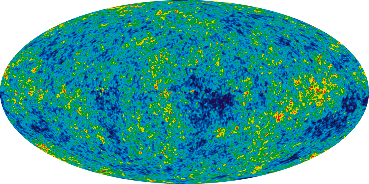
Fig. 18.5 Background radiation in the universe as observed from earth. By NASA / WMAP Science Team - http://map.gsfc.nasa.gov/media/121238/ilc_9yr_moll4096.png, Public Domain.

This radiation is the red shifted radiation from around 380,000 years after the Big Bang when the universe became transparent. At that time the temperature had dropped (due to the adiabatic expansion) to around 3000 K, at which protons and electrons can form stable hydrogen atoms \(p+e^- \to H\). This event is called recombination. At higher temperatures photons are scattered from the free electrons (and protons) constantly, effectively the photons have a very short mean free path and the universe is opaque. At the recombination temperature all of a sudden the photon could travel without strong scattering, the universe was transparent. The 3K cosmic background radiation that we measure today is the red-shifted version of this 3000 K light. It gives us a glimpse of how the universe looked at that time. Apart from the background radiation there were no other light sources in the universe as stars had not formed yet, the Dark Ages of the universe began.

The red-shift here is actually caused by the expansion of the universe itself (the universe expands causing the photons’ wavelength to expand). NB: Time in cosmology is often given in units of red-shift (e.g. the red-shift for recombination is \(z=1089\)).

”Wavelength temperature relation”

How can we relate the wavelength of electro-magnetic radiation to temperature?

Matter emits electro-magnetic radiation depending on its temperature. This relation is given by Planck’s law with which quantum mechanics started in 1900 as he considered black body radiation. The emitted spectral density per solid angle depends on the thermal energy \(kT\) and is given by

\[ u(\lambda, T) = \frac{2hc}{\lambda^5}\frac{1}{e^{hc/\lambda kT}-1} \]

Here for the first time \(h\), Planck’s constant, was introduced to quantize energy packages \(hf\) of oscillation.

Phenomenologically, the relation between the peak of the spectrum and the temperature was found by Wien already earlier to be \(\lambda_{peak} = \frac{b}{T}\) with \(b\) Wien’s constant \(b\sim 2900\ \mu m\cdot K\).

NB: If you buy a light bulb for a lamp, then a temperature is indicated on the packaging, e.g. 2700 K for “warm white”, 4000 K for “cool white” to describe the light color. Quantum physics at your local super market.

18.3. Examples

Example 18.1 21cm hydrogen line

21 cm line of hydrogen in radio astronomy. The proton and electron in the hydrogen atom both have a magnetic dipole moment related to their spin. The total quantum mechanical wave function can have 2 states for the spins, parallel or anti parallel, where anti parallel is energetically favorable. The transition between these two states is forbidden to first order (you will learn more about this in your courses on Quantum mechanics in the second and third year). By Fermi’s golden rule of quantum mechanics that means the probability that it happens per second is very small, here \(10^{-15}s^{-1}\) or that the lifetime of the excited state is very long \(\sim 10^7\) years. As space is vast and there is much hydrogen, however, this still happens a lot such that we can observe it.

Due to the very long life time, the emission line is very sharp, i.e. it has a small natural spectral broadening. This can be seen from Heisenberg’s uncertainty principle \(\Delta E \Delta t \sim \hbar\). If \(\Delta t\) is very large, then \(\Delta E\) is small and the spectral line is very sharp. Therefore shifts to this line must come from Doppler shifts which can be used to measure speeds accurately.

18.4. Exercises

Exercise 18.1

Observers \(S'\) is moving at \(V/c = 3/5\) with respect to \(S\). Both observers have their \(x\) and \(x'\) axis aligned. If they are at the same position (\(x=x'=0\)), they set their clocks to zero.

\(S'\) observes an object traveling at \(4/5\) of the speed of light in the negative \(x'\)-direction.

Calculate the velocity according to \(S\).

Exercise 18.2

Same situation as in ex.(18.1), but now \(S'\) observes that the object is moving in the \(y'\)-direction with velocity \(\frac{4}{5} c\).

Show that the magnitude of the velocity of the object according to \(S\) is smaller than \(c\).

Exercise 18.3

In order to send information via electro-magnetic waves, people use amplitude modulation (AM) and frequency modulation (FM). AM means that the amplitude of the wave that is send out varies: the variations can be detected by the receiver and ‘decoded’ to the message. FM, on the other hand, means that the frequency of the wave is changing. This can also be detected and decoded to the message.

Captain Kirk on board of the starship USS Enterprise is traveling at a speed of \(\frac{V}{c} = \frac{40}{41}\) with respect to earth. He uses FM and sends his monthly report to mission control using a center frequency of 10GHz. What is the frequency that Mission Control needs to look for in case:

1. Enterprise is moving straight towards earth;

2. Enterprise moves radially away from earth;

3. Enterprise moves tangentially to earth.

Exercise 18.4

In the year 2525 a young Applied Physics student (who doesn’t take his study to seriously) is caught ignoring a red traffic light and gets a fine. Trying to be a smarty, he refuses to pay and calls for a hearing in court.

The judge asks the student why he doesn’t want to pay: ignoring a red traffic light is dangerous and a fine is in place.

The student argues, that he wasn’t ignoring a red light: the light was clearly green.
The judge asks: “which light: the bottom one, the middle one or the top one?”

The students replies: the top one of course. I was riding my fat bike at a lovely high speed and noticed that only the top light of the traffic light was on. And it was definitely green.”

The judge has heard enough. She adjourns the session and retreats to her office. There, she picks up her notebook and calculates what the velocity of the student was. Then she calculates the fine for speeding, using the formula “fine = 5Euro * (speed (in km/h) - 40km/h)”.

She returns to the court room and the session is continued by her ruling. The student is acquitted of running a red light but is fined for speeding.

What is the amount of the fine?

18.5. Answers

Solution to Exercise 18.1

According to \(S'\) the object has velocity \(u'_{x'}/c = -4/5\). Observer \(S\) uses the velocity transformation for the \(x\)-component of velocities:

\[ \frac{u_x}{c} = \frac{\frac{u'_{x'}}{c} + \frac{V}{c}}{1+ \frac{V}{c} \frac{u'_{x'}}{c}} = \frac{\frac{-4}{5} + \frac{3}{5}}{1 - \frac{3}{5}\cdot\frac{4}{5}} = -\frac{5}{13} \]

Solution to Exercise 18.2

According to \(S'\) the object has velocity \(u'_{x'}=0\) and \(u'_{y'}/c = 4/5\). Observer \(S\) uses the velocity transformation for the \(x\) and \(y\)-component of velocities:

\[ \frac{u_x}{c} = \frac{\frac{u'_{x'}}{c} + \frac{V}{c}}{1+ \frac{V}{c} \frac{u'_{x'}}{c}} = \frac{3}{5} \]

\[ \frac{u_y}{c} = \frac{\frac{u'_{y'}}{c}}{\gamma (V) \left ( 1+ \frac{V}{c} \frac{u'_{x'}}{c} \right ) } = \frac{\frac{4}{5}}{\frac{5}{4}} = \frac{16}{25} \]

Thus the magnitude of \(\vec{u}\) is:

\[ \frac{u}{c} = \sqrt{\frac{u_x^2}{c^2} + \frac{u_y^2}{c^2}} = \sqrt{\frac{481}{625}} \approx \frac{22}{25} \lt 1 \]

Solution to Exercise 18.3

Doppler shift

\[ \frac{f_0}{f} = \frac{1+\frac{u_r}{c}}{\sqrt{1-\frac{u^2}{c^2}}} \]

In this case: \( u/c = 40/41 \rightarrow \gamma = \frac{41}{9} \)

1. \(u_r/c=-40/41 \rightarrow \frac{f_0}{f} = \frac{1}{41}\frac{41}{9} \rightarrow f=9f_0 = 90GHz\)

2. \(u_r/c=40/41 \rightarrow \frac{f_0}{f} = \frac{81}{41}\frac{41}{9} \rightarrow f=\frac{1}{9}f_0 = 1.11GHz\)

3. \(u_r/c=0 \rightarrow \frac{f_0}{f} = \frac{41}{9} \rightarrow f=\frac{9}{41}f_0 = 2.20GHz\)

Solution to Exercise 18.4

Obviously, the student tries to claim that due to his high speed, the red color of the traffic light was green to him. As he is approaching the light source, with a velocity \(V/c\), he may also take the point of view of an observer in a frame in which he is not moving, but the traffic light is approaching with \(V/c\),

The wave length of red light is 630nm and of green light 530nm. Or in terms of the corresponding frequencies: \(f_r = \frac{c}{\lambda_r} = 4.76 \cdot 10^{14}\)Hz and \(f_g = 5.66 \cdot 10^{14}\)Hz. In the rest frame of the traffic light, the frequency is thus: \(f_0 = f_r\), whereas in the frame of the student it is \(f=f_g\).

If we plug this into the Doppler shift formula, we get:

\[\begin{split}\begin{split} \frac{f_0}{f} = \frac{f_r}{f_g} = 0.82 = \frac{1+\frac{u_r}{c}}{\sqrt{1-\frac{u^2}{c^2}}} = \sqrt{\frac{1+V/c}{1-V/c}} \Rightarrow\\ \frac{1+V/c}{1-V/c} = 0.68 \rightarrow \frac{V}{c} = 0.2 \end{split} \end{split}\]

Thus the biker claims to have a speed of 20% of the speed of light, that is 2.16 10\(^8\) km/h and accordingly gets a fine of 1.08 billion Euro.