13. Rigid Body

Note: Students find the motion of the rigid body the most difficult part of the course. Be warned.

13.1. Finite-Sized Objects

Newtonian mechanics is, in its beginning, a theory for point particles. In some instances, reducing an extended object to a point is allowed e.g. when considering the gravity exerted by a spherical object like the Sun and we can picture the Sun as a point with the total mass concentrated there. In many practical cases, however, it is not a good approximation.

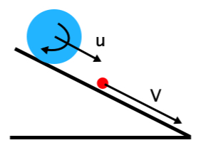
Fig. 13.1 A ball and a point mass on a slope.

For example, think of a ball rolling down a slope and compare its motion to the frictionless sliding of a point particle along the slope. You will find that the rolling ball is slower than the sliding particle. Note that rolling always means that there must be some form of friction, otherwise the object would not roll, but slide.

That the rolling ball is slower, is not a surprise if we consider the energy of both objects: the sliding point particle loses potential energy and gains an equal amount of kinetic energy (ignoring friction). The rolling ball, of course, also loses potential energy and gains kinetic energy. But it has to split this kinetic energy over kinetic energy associated with its translation and that associated with its rotating. Consequently, it has less kinetic energy of translation and thus translates with a lower velocity than the point particle.

In the animation below, you will see a point particle sliding down the slope, without friction, a massive disc rolling down and a wheel rolling down. All objects have the same mass \(m\). The wheel and disc have radius \(R\). They start from the same position without velocity.

Fig. 13.2 A wheel, disc and a point mass on a slope.

Clearly, the point particle moves fastest, followed by the disc and then the wheel. How can we model this? In what follows, we will find a way.

13.2. Constraining Forces

We have seen that the total momentum of a many-body system responds only to external forces. All internal forces, i.e., from one of the particles to another, always have a corresponding opposite force thanks to N3 action = -reaction. We don’t need to know the details of these interaction forces to understand the motion of the center of mass.

We can exploit this by assuming that the interaction forces in a rigid body are such that they keep the relative position of the particles fixed at all times. I.e. the object’s shape cannot change, it is called rigid. We can translate it, we can rotate it. But we cannot deform it - change the relative position of the particles that make up the object. This is something that we can apply to our mechanical problems in daily life. Most objects don’t change shape if we put a force on them. Or put somewhat better: the change of shape is unnoticeable to us. In reality, there must be a small change in shape (causing acoustical waves) and the atoms making up a solid body always vibrate a bit as by their thermal energy.

So, from here on we replace the true interparticle forces by the constraints. All these constrains do, is keeping the relative position of the particles fixed. We do not try to describe them. As we will see below, we don’t need any information of these fictitious forces.

13.3. Angular Velocity and Acceleration

Our rigid body can do two things: translate and rotate. Rotation is always around some axis. This axis can be indicated by a vector. By assigning to the axis a vector property we can implicitly define the rotation direction (clockwise/ counter clockwise) around the axis, otherwise it would not matter for the rotation axis if it points up or down. This axis can be fixed in space (e.g. a spinning wheel on a fixed axis) or change as a function of time, the rotation axis rotates itself around another axis (e.g. a spinning top at an angle to the normal) or translates like that of the rolling wheel and disc in the above animation.

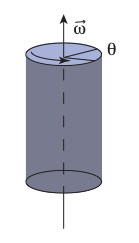
Fig. 13.3 Rotation axis and definition of rotation angle and angular velocity.

For the moment we only consider rotation about a fixed axis, see figure. We can describe the positions of all particles constituting the cylinder by specifying the location of its center of mass, the direction that the axis is pointing, and the angle of rotation \(\theta\) around the axis.

As the angle \(\theta(t)\) can change in time, we also need to consider the rate of change, the angular velocity.

\[ \omega \equiv \frac{d \theta}{dt} \]

However, this does not tell us anything about the orientation of the axis around which the cylinder is rotating. For a given \(\omega\) the axis can point in any direction. It is like telling you the magnitude of the velocity of an object but not giving you any clue in which direction that object is moving.

We can easily cure this by realizing that \(\omega\) actually has a direction, like velocity. If we treat it like a vector, the direction of the vector will give us the orientation of the rotation axis. Thus, from now on, we will use the angular velocity vector \(\vec{\omega}\). Here the right hand rule applies. Use your thumb in the \(\vec{\omega}\) direction to determine the direction of positive rotation in the direction of the other fingers. I.e. if the thumb is sticking up, counter clockwise is the positive direction.

The vector angular acceleration is:

\[ \vec{\alpha} \equiv \frac{d \vec{\omega}}{dt} \]

The relation between the angular velocity \(\vec{\omega}\) and the linear velocity of a particle \(s\) that is part of the rigid body, is given by

\[ \vec{v}_s = \vec{\omega} \times \vec{r}_s \]

as the angular velocity is the same for all particles and the linear velocity must increase with distance from the rotation axis \(\vec{r}_s\). Please note the vector character of this equation. All the quantities are vectors and the cross product relates them.

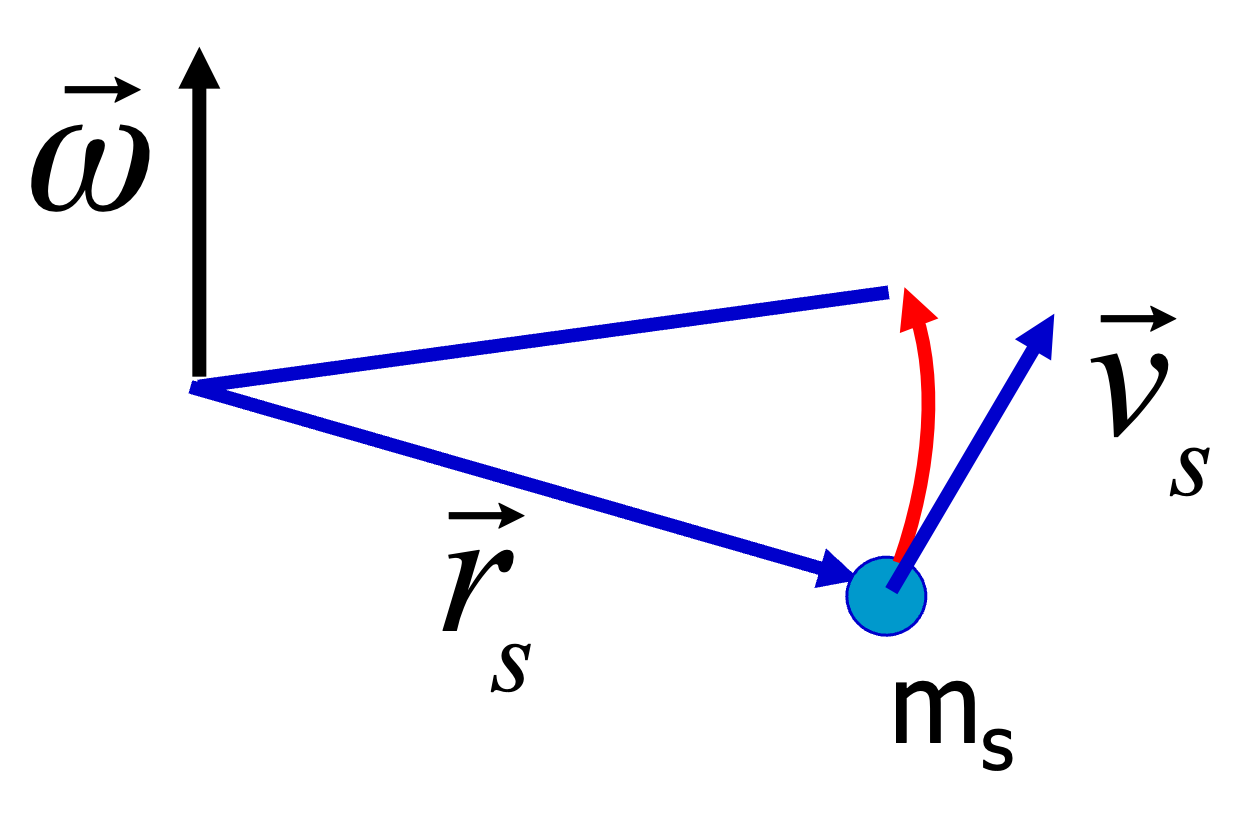
Fig. 13.4 Relation between velocity and angular velocity of a small part of a rotating rigid body.

In general, for a N body problem, the particles do not have the same angular velocity and the above equation should also have a subscript \(s\) at \(\vec{\omega}\). However, we have replaced all mutual forces by fictitious constraint. These make sure that all relative positions stay the same. And that has as consequence, that all parts of the rigid body must rotate with the same angular velocity. We will see below, that this has far reaching consequences, making it possible to deal with many-body systems in a way analogous to our treatment of point particles.

13.4. Moment of Inertia

Now, we consider the angular momentum of one particle \(s\) (being part of our rigid body):

\[\vec{l}_s=\vec{r}_s \times \vec{p}_s = \vec{r}_s \times m_s(\vec{\omega}\times \vec{r}_s)=m_sr^2_s\vec{\omega}\]

For the total angular momentum of our rigid body we find

\[ \vec L = \sum \vec{l}_s = \sum m_s r^2_s \vec{\omega} \]

with \(\vec{\omega}\perp \vec{r}_s\). Again, because we are dealing with a rigid body, there is no subscript \(s\) on \(\vec{\omega}\): all particles of the rigid body rotate with the same angular velocity. Thus we can write: $\(\vec L = \left ( \sum m_s r^2_s \right ) \vec{\omega}\)$

The sum over the mass and positions is called moment of inertia

\[ I\equiv \sum m_s r^2_s = \int_M r^2 \, dm \]

13.5. Examples

Example 13.1 Dumbbell

Consider a dumbbell formed by a 2 masses: \(m_1= \frac{2}{3}M\) and \(m_2 = \frac{1}{3}M\) connected by a massless rod of length \(L\).

What is the moment of inertia of this dumbbell for rotation around an axis through its center of mass as shown in the figure below?

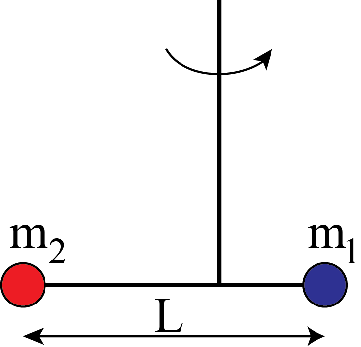
Fig. 13.5 Dumbbell rotating around an axis through its center of mass.

First, we need to find the position of the center of mass. It will be located somewhere on the massless rod. If we call the center of mass the Origin and use coordinate \(r_1\) for \(m_1\) and \(r_2\) for \(m_2\), we have:

\[m_1 r_1 + m_2 r_2 = 0 \]

Combine this with \(m_1= \frac{2}{3}M\) and \(m_2 = \frac{1}{3}M\) and \(r_1 - r_2 = L\), we get

\[ r_1 = \frac{1}{3}L \text{ and } r_2 = \frac{2}3{}L \]

Now we can calculate the moment of inertia for rotation about the given axis:

\[ I \equiv \sum_s m_s r_s^2 = \frac{2}{3}M \left [ \frac{1}{3} L \right ]^2 + \frac{1}{3}M \left [ \frac{2}{3} L \right ]^2 = \frac{2}{9} ML^2\]

The moment of inertia is a characteristic property of the shape and mass distribution of a specific solid body. It represents its resistance against change in rotation speed around a certain axis, as we see here:

\[ \vec L = I \vec{\omega}\quad \& \quad\dot{\vec{L}} = \vec{r} \times \vec{F} = \vec{\Gamma}_{ext} \]

Now we see the analogy to N2 (\(m\dot{\vec{v}}=\vec{F}\)):

\[ I\dot{\vec{\omega}} = \vec{\Gamma} \]

Thus \(I\) takes over the role of the mass \(m\) as the object property resisting a change in motion. The unit of \(I\) is [kg m\(^2\)], of \(\dot{\vec{\omega}}\) is [1/s\(^2\)] and of \(\Gamma\) is [kg m\(^2\)/s\(^2\)].

In the absence of an external torque, \(\Gamma =0\), it follows that \(\dot{\vec{\omega}}=0\), i.e. the angular velocity stays constant in magnitude and direction. The rotation axis remains constant. This is in complete analogy to N2 and N1. As an example think about earth’s rotation axis. To first order there is no external torque, therefore the rotation axis remains inclined while the earth orbits the sun. In turn this leads e.g. to different seasons away from the equator.

The moment of inertia is a property with respect to the rotation around a given axis. We will specify the quantity always with respect to one specific rotation axis. You can avoid this specification if you compute the moment of inertia for “all axis at the same time”. It is clear that \(I\) cannot be a scalar property then. From \(I\dot{\vec{\omega}} = \vec{\Gamma}\) we see that if we apply a vector (\(\vec{\omega}\)) to \(I\), then it must return a vector (\(\vec{\Gamma}\)), therefore \(I\) needs to be a “second rank tensor”. Click here for more information, if you are interested.

The equation relating the angular momentum to the angular velocity via the moment of inertia \(\vec L = I \vec{\omega}\), assumes that we are in the CM system. If that is not the case, the equation needs an extra term to include the angular momentum of the CM

\[ \vec{L} = \vec{R} \times \vec{P} + I_{CM}\vec{\omega} \]

13.5.1. Parallel axes theorem

This theorem (also known as Steiner’s theorem) lets you compute the moment of inertia \(I'\) through an axis parallel to an axis through the CM (of which you know the moment of inertia \(I\)) with distance \(d\). Consider the situation as in the sketch.

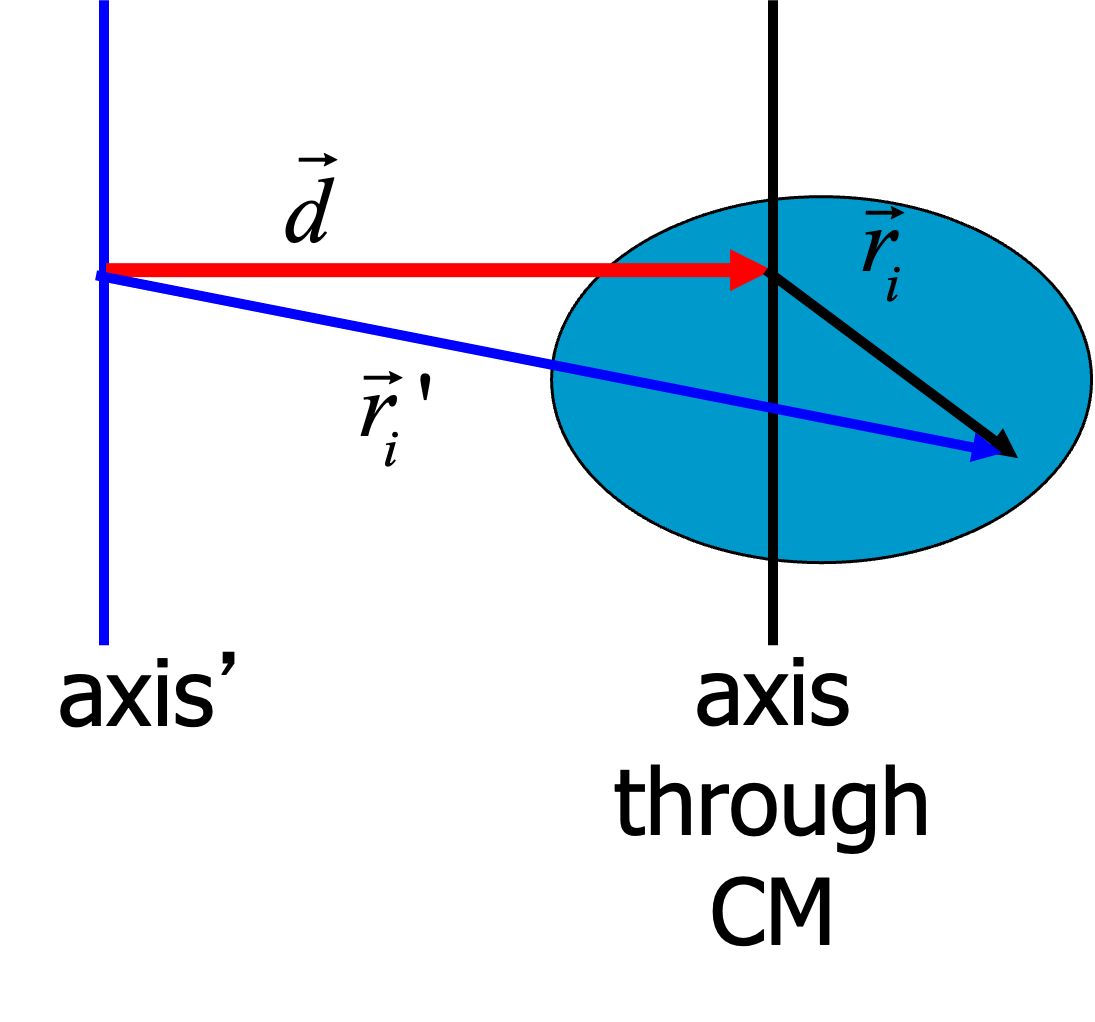
Fig. 13.6 Steiner’s theorem or the parallel axes theorem.

We are going to compute the moment of inertia around the primed axis.

\[\begin{split} \begin{array}{rcl} I' &= &\sum m r_i^{'2}=\sum m_i(\vec{d}+\vec{r}_i)\cdot (\vec{d}+\vec{r}_i)\\ &=& \sum m_i d^2 + \sum 2m_i \vec{d}\cdot \vec{r}_i + \sum m_i r^2\\ &=& Md^2 + 2\vec{d} \cdot \sum m\vec{r}_i + \sum m_i r_i^2\\ &=& Md^2 + I_{CM} \end{array} \end{split}\]

The term \(\sum m\vec{r}_i=0\) by definition of the relative positions in the CM frame and the last term is just the moment of inertia through an CM axis.

13.6. Example

13.2 Rotating Square

Consider a thin square of mass \(M\) with sides \(a\). The thickness \(\delta\) is much smaller than \(a\): \(\delta \ll a\). The density of the square, \(\rho\), is a constant.

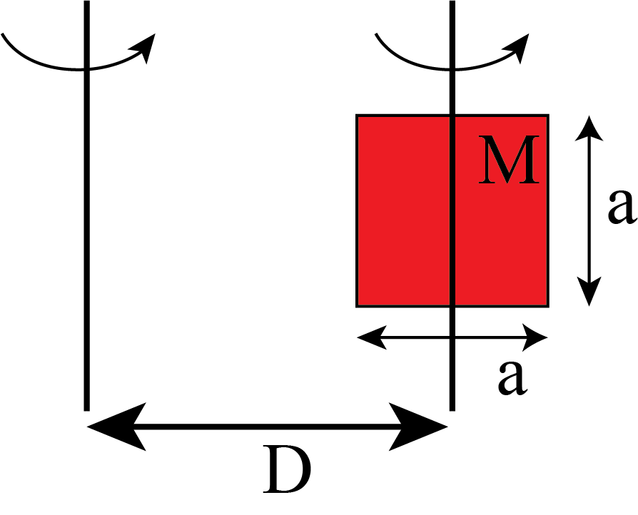
Fig. 13.7 A thin square rotating around an axis through its center of mass or around one that is shifted over a distance \(D\).

Find the moment of inertia for rotation around an axis through the center of mass of the square as shown in the figure. And find the moment of inertia for rotation around the second axis, that is displaced over a distance D.

Solution 13.2

The center of gravity of the square is located at the square’s center (density is constant and we use symmetry). Thus the moment of inertia \(I_{CM}\) calculated as follows:

\[\begin{split}\begin{split} I_{CM} &\equiv \sum_s m_s r_s^2 \\ &= \int_{-a/2}^{a/2} \int_{-a/2}^{a/2} r^2 dm \\ &= \int_{-a/2}^{a/2} \int_{-a/2}^{a/2} x^2 \rho \delta dxdy \\ &= \rho \delta \int_{-a/2}^{a/2} dy \int_{-a/2}^{a/2} x^2 dx \\ &= \rho \cdot a \cdot \left [ \frac{1}{3} x^3 \right ]_{-a/2}^{a/2} \\ &= \frac{1}{12}Ma^2 \end{split}\end{split}\]

The moment of inertia om the second axis is now readily obtained via Steiner’s theorem:

\[ \begin{split} I' = I_{CM} + MD^2 = M \left ( D^2 + \frac{1}{12}a^2 \right ) \end{split} \]

13.6.1. Radius of Gyration

The radius of gyration \(R_G\) is defined by assigning an easy to visualize (and comparable) moment of inertia to an irregular shaped object with known moment of inertia \(I\) and mass \(M\). The moment of inertia of a point mass \(M\) at distance \(R\) from the rotation axis is \(MR^2\) of course, therefore we can define the radius of gyration

\[ R_G = \sqrt{I/M} \]

This gives you at what distance from the rotation axis a point of the same mass has an equivalent moment of inertia. For example in biophysics this is used to describe the dimensions of a polymer chain.

13.7. Kinetic Energy of Rotation

We can computed the kinetic energy of rotation from \(E_{kin} = \sum \frac{1}{2} m_s v^2_s = \sum \frac{1}{2} m_s \vec{v}_s\cdot \vec{v}_s\) and substituting \(\vec{v}_s = \vec{\omega} \times \vec{r}_S\)

\[ E_{kin} = \sum \frac{1}{2} m_s r^2_s \omega^2 = \frac{1}{2}I\omega^2 \]

under the assumption \(\vec{\omega} \perp \vec{r}\), i.e. the moment of inertia \(I\) corresponds to the rotation around the axis given by \(\vec{\omega}\). Again this can be generalized to rotations around any axis, but requires then the introduction of the inertia tensor such that \(E_{kin}=\frac{1}{2}\vec{\omega} \cdot \bf{I} \cdot\vec{\omega}\) remains a scalar.

Please notice the analogy to the kinetic energy of linear motion \(\frac{1}{2}mv^2\), the linear velocity is replaced by the angular velocity and the mass by the moment of intertia. Exactly what you would expect.

13.8. Gyroscope & Precession

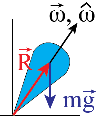
Fig. 13.8 Spinning top

Rotating bodies are of large interest as the earth itself is rotating, but also technically for gyroscopes. Here we consider a spinning top. Although this is a children’s toy, the physics are quite involved. The description of the motion of the earth around the sun is governed by the same ideas. Note that the rotation axis of the earth is inclined to the plane it moves around the sun by 23.5 degrees, but as there is no external torque to first approximation, the axis remains stable while the earth circles the sun (due to \(I\dot{\vec{\omega}}=\vec{\Gamma}=0\)). This leads e.g. to different seasons on the northern and southern hemisphere. To second order there is a small torque due to the non-uniformity of gravitational field from the sun and the moon on the earth, resulting a similar motion as for the spinning top under the influence of gravity.

Looking at the figure of the spinning top under the influence of gravity we see the there is a torque applied to the system.

\[ I\dot{\vec{\omega}}= \vec{\Gamma} = \vec{R}\times m\vec{g} \]

The rotation axis is parallel to \(\vec{R}\), therefore \((\vec{R}\times m\vec{g}) \perp \vec{\omega}\)

\[\begin{split} \begin{array}{l} \Rightarrow \vec{\omega} \cdot I\dot{\vec{\omega}}=\vec{\omega}\cdot (\vec{R}\times m\vec{g}) = 0\\ \Rightarrow \vec{\omega} \perp \dot{\vec{\omega}}\\ \frac{1}{2}\frac{d}{dt}\vec{\omega}^2=\vec{\omega}\cdot\dot{\vec{\omega}}=0\\ \Leftrightarrow \|\vec{\omega}\| = const. \end{array} \end{split}\]

We find that the angular velocity remains constant in magnitude and only the direction can change! Therefore the axis \(\hat{\omega}\) must move in a circle (around the normal); the axis describes a cone in space. This type of motion is called precession. See here for a movie of precessing gyroscope.

If we now want to write down the equations of motion for the spinning top, we write \(\dot{\vec{\omega}}=\omega_0 \dot{\hat{\omega}}\) as only the direction changes.

\[\begin{split} \begin{array}{rcl} I\omega_0 \dot{\hat{\omega}} &=& R\hat{\omega} \times (-mg\hat{z})\\ \Rightarrow \dot{\hat{\omega}} &=& \frac{mgR}{I\omega_0} \hat{z} \times \hat{\omega} = \vec{\Omega}_p \times \hat{\omega} \end{array} \end{split}\]

with the precession frequency \(\vec{\Omega}_p = \frac{mgR}{I\omega_0} \hat{z}\) around the \(z\)-axis\( as seen by \)\hat{z}$. Next, we spell out the cross product in its components

\[\begin{split} \begin{array}{rcl} \frac{d}{dt}\hat{\omega}_x &=& -\Omega_p \hat{\omega}_y\\ \frac{d}{dt}\hat{\omega}_y &=& +\Omega_p \hat{\omega}_x\\ \frac{d}{dt}\hat{\omega}_z &=& 0 \end{array} \end{split}\]

Eliminating either the \(x\) or the \(y\) component gives a differential equation for the axis components

\[ \frac{d^2}{dt^2}\hat{\omega}_x + \Omega_p^2 \hat{\omega}_x =0 \]

with (harmonic) solution

\[ \hat{\omega}_x (t) = A \sin (\Omega_p t) + B \cos (\Omega_p t) \]

Now we again see that the \(\vec{\omega}\) axis rotates with angular frequency \(\Omega_p\) around the \(\hat{z}\) axis. As \(\frac{d}{dt}\hat{\omega}_z = 0\) the height of the axis remain stable, and it moves over a cone. We can see that the larger \(\omega_0\), the smaller \(\Omega_p\) and the more stable the gyroscope will be. (Ask yourself: What do we mean with stable here? And why is this the case?) The opening angle of the cone is given by the initial tilt of the spinning top - it does not change under the influence of gravity. Gravity only induces the precession (a motion perpendicular to the action of the gravity via the torque).

As the gravitational pull of the sun and moon on the earth is not uniform, also the earth experiences a torque and precesses. The precession periode of the earth is very long compare to modern human history with 26,000 years, but short compared to geological times.

13.9. Comparison linear & rotational motion

\[\begin{split} \begin{array}{lll} \text{moment of inertia }&I & \text{mass }m\\ \text{torque}& \vec{\Gamma}=\vec{r}\times\vec{F} & \text{force } \vec{F}\\ \text{angular momentum}&\vec{L}=I\vec{\omega} & \text{momentum } \vec{p}=m\vec{v}\\ \text{equation of motion}& \vec{\Gamma}=I\dot{\vec{\omega}}=\dot{\vec{L}} & \vec{F}=m\dot{\vec{v}}=\dot{\vec{p}} \\ \text{work}& dW=\vec{\Gamma}\cdot d\theta & dW=\vec{F}\cdot ds\\ \text{energy}&E_{kin}=\frac{1}{2}I\omega^2 & E_{kin}=\frac{1}{2}mv^2\\ \end{array} \end{split}\]

13.10. Worked Examples

Example 13.3

Calculate the moment of inertia of a massive cylinder, constant density, length \(L\) with outer radius \(b\) and inner radius \(a\) that is rotating around the long axis.

Fig. 13.9 Hollow cylinder rotating around its long axis

Definition of moment of inertia:

\[ I=\int_M r^2\, dm \]

First transform the mass element \(dm\) into a volume element \(dm=\rho dV\). Note that the density \(\rho\) may be a function of \(\vec{r}\).

The volume element in cylindrical coordinates, with \(r\) the distance from the rotation axis is \(dV = L 2\pi r \, dr\). This gives for the moemnt of inertia:

\[ I = 2\pi \rho L \int_a^b r^3\,dr = 2\pi \rho L \frac{1}{4}(b^4-a^4) \]

Now we can simplify this by bringing in the total mass of the object, here that is \(M=\rho L\pi (b^2-a^2)\). We obtain

\[\begin{split} \begin{array}{rcl} I &=& \frac{1}{2}M(b^2+a^2) \\ I_{full} &=& \frac{1}{2} MR^2 \;\;\;\;\;\;\;\;\;\;\;\;\;\; (a=0)\\ I_{thinwall}&=& MR^2 \;\;\;\;\;\;\;\;\;\;\;\;\;\;\;\; (a=b) \end{array} \end{split}\]

Notice that a thin walled cylinder has a higher moment of inertia than a full cylinder of the same mass. That is because the distribution of the mass with respect to the rotation axis matters!

Example 13.4

A solid round disk is hanging from the ceiling suspended via a massless rod. The system is oscillation around the equilibrium position just as with the pendulum treated earlier. What is the oscillation frequency?

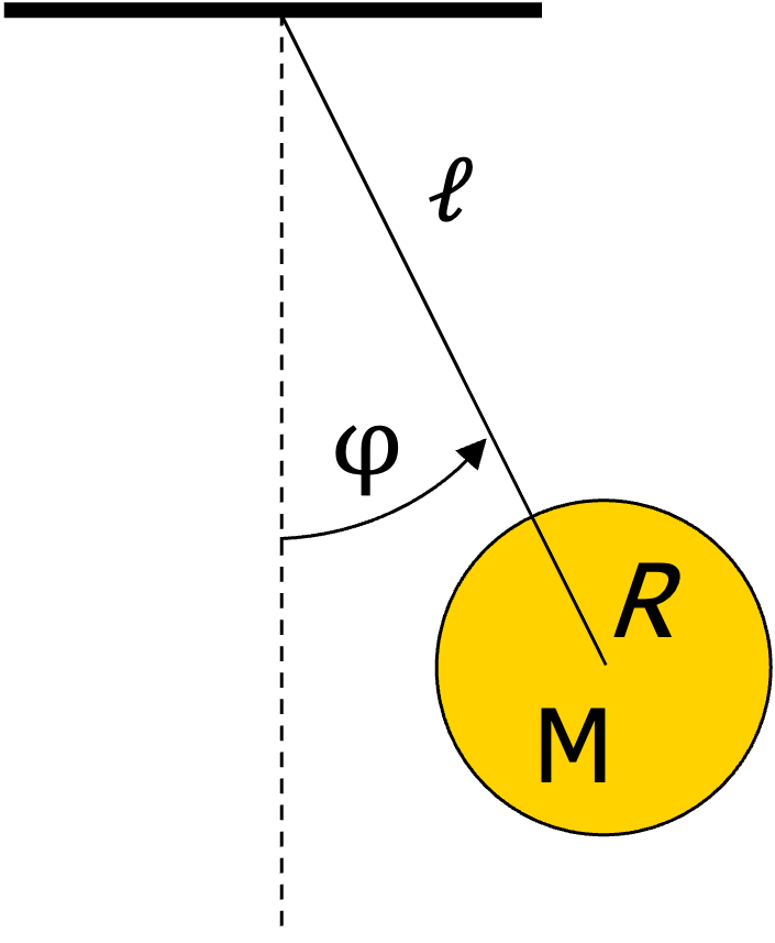
Fig. 13.10 pendulum with disk

If we want to derive the equation of motion for the system, we need to setup “N2” for rotation

\[ I\dot{\vec{\omega}} = \sum \vec{\Gamma} = \vec{x} \times \vec{F}_g \]

The torque applied by gravity is pulling the disk inward and we have \(\vec{x} \times \vec{F}_g = -\ell Mg\sin\varphi\). Furthermore, we see that the disk (with \(I_{CM}=\frac{1}{2}MR^2\) just think of the disk as a very flat full cylinder for which we calculated the momentum of inertia above) is rotating not around an CM axis (which is perpendicular to the screen plane), but around an axis perpendicular to the screen through the pivot point. This axis is parallel to the CM axis and we can apply Steiner’s theorem to compute the appropriated moment of inertia as

\(I=M\ell^2+I_{CM} = M\ell^2 + \frac{1}{2}MR^2\).

Substituting these findings into “N2” together with \(\omega=\dot{\varphi}\), we obtain

\[ (M\ell^2 + \frac{1}{2}MR^2) \ddot{\varphi}+\ell Mg \sin\varphi =0 \]

If you compare this to the equation of motion we obtained earlier for the pendulum only the extra term \(\frac{1}{2}MR^2\) has entered accounting for the moment of inertia of the disk.

From the above equation, we immediately get the oscillation frequency for small angles (\(\sin \varphi \approx \varphi\)):

\[ \omega_0^2 = \frac{\ell g}{\ell^2 + \frac{1}{2}R^2} = \frac{1}{1+\frac{1}{2}\frac{R^2}{\ell^2}}\frac{g}{\ell}\]

Example 13.5

We will compute the moment of inertia of a solid sphere, radius \(R\) and mass \(M\) (constant density). There are two approaches a) via setting up the problem in spherical coordinates and the volume element or b) via sectioning the sphere into thin disks of different radii.

1. Via the volume element.

Fig. 13.11 Moment of inertia of a sphere: volume element

Realize that \(r\) is the distance to the rotation axis and \(s\) is the distance to the volume element \(dV\) (typically many mistakes happen in this step), therefore the volume element is given by \(dV=s^2 \sin\theta \,ds d\theta d\varphi\)

\[\begin{split} \begin{array}{rcl} I&=&\displaystyle{\rho \int_V r^2 \,dV = \rho \int_V d\varphi\, d\theta \sin \theta \, ds\, s^2 (s \sin\theta)^2}\\ &=&\displaystyle{\rho \int_0^{2\pi} d\varphi \int_0^\pi d\theta \sin^3 \theta \int_0^R ds\, s^4}\\ &=& \rho 2\pi \frac{4}{3}\frac{1}{5}R^5 = \frac{2}{5}MR^2 \end{array} \end{split}\]

This approach only works if you can evaluate the finite integral over \(\sin^3\theta\) which is not straight forward, but doable (and it is equal to \(4/3\)).

2. In the second approach, we slice the sphere in thin disks (\(I_{disk}=\frac{1}{2}MR^2\)) as shown in the figure

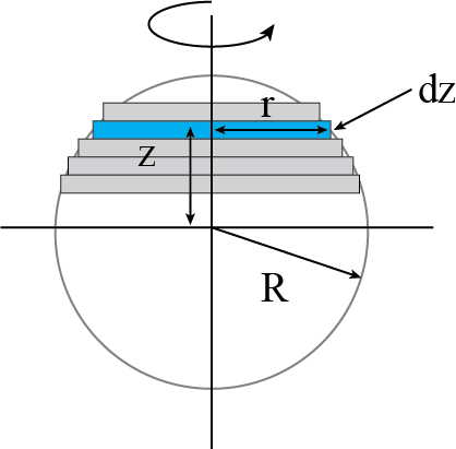
Fig. 13.12 Moment of inertia of a sphere: slice element

We now have to add all disks, that is \(I_{sphere} = \sum I_{disc}\). By making the discs very thin, i.e. \(dz\rightarrow 0\), the sum will go over to an integral. Moreover, instead of \(I_{disc}\) we will write \(dI_{disc}\). The integration will run from the lowest disc at \(z=-R\) to the top one at \(z=R\).

\[ I=\int_V r^2\, dm=\int_{-R}^{+R} dI_{disk} \]

The distance to the rotation axis is \(r\) and we integrate over \(z\). Now we have to specify how \(r\) varies with \(z\). That follows from Pythagoras: \(z^2 + r^2 = R^2\)

Moreover, we explicitly have to write \(dI_{disc}\) in terms of \(dz\). That goes by realizing, that \(dI_{disc} = \frac{1}{2}dM r^2\), where \(dM\) is the mass of a disc. This is also a function of \(z\):

\[dM = \rho dV = \rho \pi r^2 dz \]

Hence for the contribution of a disc, we can write:

\[ dI_{disk} = \frac{1}{2}r^2dM = \frac{1}{2}r^2 \pi\rho r^2\,dz = \frac{1}{2} \pi \rho r^4 dz \]

This gives us a much easier integral to solve now and we arrive at the same result as before

\[ I = \frac{1}{2}\rho\pi \int_{-R}^{+R} r^4\,dz = \frac{1}{2}\rho\pi \int_{-R}^{+R} (R^2-z^2)^2\,dz =\frac{2}{5}MR^2 \]

Example 13.6

A massive cylinder mass \(M\), radius \(R\) is rolling down an inclined slope (inclination angle \(\theta\)) without slipping. Compute the linear acceleration down the slope.

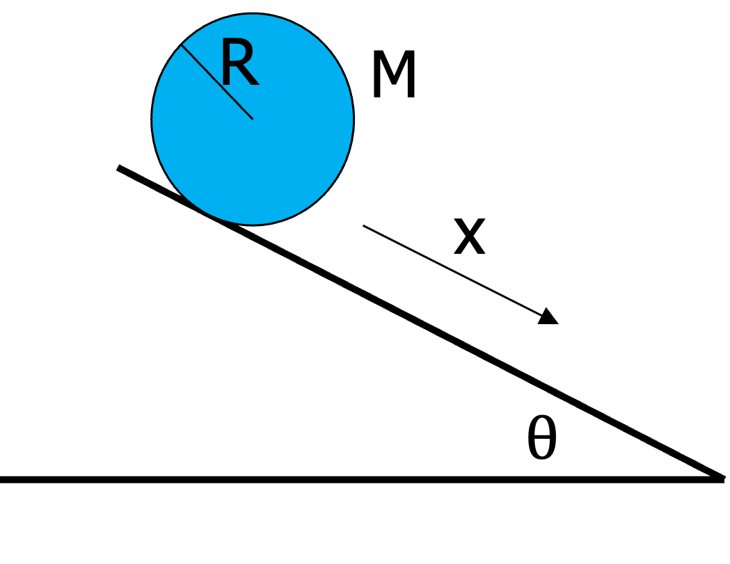
Fig. 13.13 A cylinder rolling down a slope.

There are several ways towards the solution and we will follow the idea of energy conversation (such that we do not need to worry too much about the forces/torque). Other approaches are via the friction force and torque from \(\vec{F}=m\vec{a}\) and \(\vec{\Gamma}=I\dot{\vec{\omega}}\) or directly via the torque around the point where the cylinder touches the slope.

If the cylinder is rolling without slipping, its angular and linear velocity are related as \(v=\omega R\).

The total energy is given by

\[ E=\frac{1}{2}Mv^2+\frac{1}{2}I\omega^2+Mgh \]

That is, it is the sum of kinetic and potential energy from gravity. Why don’t we account for the work done by the friction force? Is there a friction force? To start with the second question: yes, there must be a friction force otherwise the cylinder would slip and not roll down the slope. But this friction force dows not perform work! In the case we are considering, rolling means that the point of contact of the cylinder with the slope has zero velocity. At the point of contact, the translation via the motion of the center of mass is exactly compensated by the angular velocity. And thus the momentary displacement of this point is zero: friction can not perform work on it as that requires \(\vec{F}_f \cdot d\vec{s}\) and the latter is zero!

The moment of inertia of a massive cylinder is \(I=\frac{1}{2}MR^2\). If the cylinder moves down over a distance \(x\) the height is lowered by \(x \sin\theta\).

\[ E = \frac{1}{2}Mv^2+\frac{1}{2}\frac{1}{2}MR^2 \left ( \frac{v}{R} \right )^2 -Mgx\sin\theta \]

Now invoking conservation of energy we take the time derivative of this expression to obtain

\[ Mv\dot{v}+\frac{1}{2}Mv\dot{v}-Mgv\sin\theta = 0 \]

Here we can divide out the mass \(M\) and the velocity \(v\) as it is non-zero, to obtain

\[ a+\frac{1}{2}a-g\sin\theta=0 \Rightarrow a = \frac{2}{3}g\sin\theta \]

The acceleration is smaller than for a point mass. You can reason this as some energy needs to be transferred to rotating the cylinder, but that is not needed for a point mass. For the latter the acceleration is simply \(g\sin\theta\).

N.B. You are faster down a hill if you slip e.g. on skis than you are with your bike (without pushing the pedals). We have here ignored air friction. Friction does act on the bikers wheels, but not on the skis. How big is the frictional force on the cylinder in the above example? Try to derive that yourself.

Example 13.7

Two masses sliding on a rotating stick

We have the following situation. A stick with two masses \(m\), located at the end of a stick of length \(2R\), is rotating. In the center of the stick are two smaller masses of \(m/2\). Initially they are in the center (situation 1), but as the stick is rotating with \(\omega_1\) they move to the outside and join the other masses (situation 2).

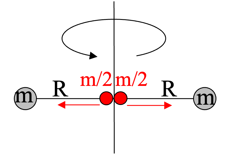
Fig. 13.14 Rotating stick: two particles at the center (situation 1).

What is the rotation speed \(\omega_2\) in situation 2 after the masses of \(m/2\) moved to the side?

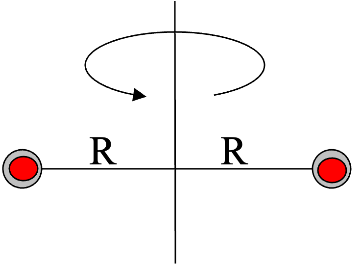
Fig. 13.15 Rotating stick: all particles at the end (situation 2).

Because there are only internal forces and torques and no external ones, the total angular momentum is conserved.

\[\begin{split} \begin{array}{rcl} \vec{L}_1 &=& \vec{L}_2 = \vec{r}\times \vec{p}\\ \Rightarrow 2\cdot R\, m \omega_1 R &=& 2\cdot R\; \frac{3}{2}m \omega_2 R \end{array} \end{split}\]

Thus we find \(\omega_2 = \frac{2}{3}\omega_1 < \omega_1\).

Is \(E_{kin}\) conserved here?

No. The masses \(m/2\) do not magically move to the side. It may look as the stick is rotating, but if you place yourself into the frame of the stick, you see directly that work needs to be done to move the small masses to the side. Thus the kinetic energy in situation 2 is smaller than in situation 1. Therefore solving for the rotation speed via \(\frac{1}{2}I_1\omega_1^2 = \frac{1}{2}I_2\omega_2^2\) is not correct.

Example 13.8 Atwood machine

An Atwood machine consists out of a pulley, sometimes considered massless, over which a string is connected to two masses. Here we consider the pulley as a solid disk with mass \(M\) and radius \(R\), having a moment of inertia \(I=\frac{1}{2}MR^2\) (Check if you can compute this simple moment of inertia easily by now). The string is massless.

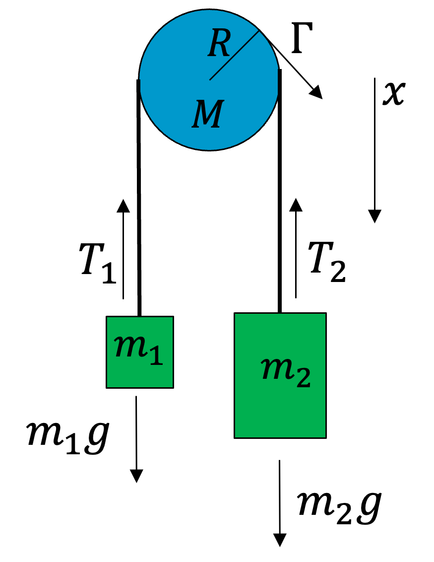
Fig. 13.16 Atwood machine

Task: Compute the acceleration on the two masses.

First, we need to recognize that the positions, velocities and accelerations of the two masses are connect to each other, but also to the pulley via the string. If mass 2 goes down with acceleration \(\vec{a}\) then mass 1 goes up with \(-\vec{a}\). The angular acceleration of the pulley is \(\alpha = a/R\) and is also connected to the motion of the masses, if the string is not slipping.

We solve for the acceleration by considering gravity, the forces in the string \(T_1,T_2\) and the torque \(\Gamma\) on the pulley.

We chose the positive \(x\) axis pointing down as \(m_2>m_1\). Then the angular acceleration is also positive, as is the torque. The forces acting on the masses and the torque on the pulley are

\[\begin{split} \begin{array}{rcl} m_1g-T_1 &=& -m_1a\\ m_2g-T_2 &=& m_2a\\ \Gamma = (T_2-T_1)R &=& I \alpha =\frac{1}{2}MR^2\frac{a}{R} \end{array} \end{split}\]

Note that we used here that the string is massless.

Solving the first two equations for \(T_1\) and \(T_2\) and substituting in the third, we obtain

\[ m_2(g-a)-m_1(g+a) = \frac{1}{2}Ma \]

and after solving for the acceleration \(a\)

\[ a= g\frac{m_2-m_1}{m_2+m_1+\frac{1}{2}M} \]

We can verify that for \(m_1,M\to 0 \Rightarrow a=g\) which makes sense and also \(0<a<g\). Also \(m_1=m_2 \Rightarrow a=0\). Check.

NB: For the case of a massless pulley you can directly solve with \(T_1=T_2\).

Via the conservation of energy:

Of course you can obtain the same result via the total energy:

\[ E= \frac{1}{2}m_1v_1^2 + \frac{1}{2}m_2v_2^2 + \frac{1}{2}I\omega^2 +m_1g(H-x) + m_2 g (H+x) \]

Now we use \(v_1 = -v_2\) and rolling without slipping condition \(\omega=v/R\) together with \(I=\frac{1}{2}MR^2\) which gives the same acceleration as above after differentiation with respect to time.

13.11. Demos & Examples

1. Flywheels are large, heavy rotating disk that can story very large amounts of energy in their rotation and e.g. release them very quickly for the generation of high currents or magnetic fields for nuclear fusion experiments. Let’s put some numbers to it. For a wheel of \(R=2\) m and mass \(M=200\cdot 10^3\) kg, rotation at a speed of 1800 rpm (=30 1/s), the kinetic energy stored is \(E=\frac{1}{2}I\omega^2=\frac{1}{4}200\cdot 10^3\cdot 2^2\cdot 30^2= 180\) MJ (or 50 kWh) but can be released in seconds.

2. The complicated physics of a rotating bicycle wheel by Prof. Walter Lewin from MIT starting from 14:30.

3. Practice your thinking about (angular) momentum and energy by shooting a bullet into a piece of wood.

4. Watch a gyroscope in space.

13.12. Exercises

Exercise 13.1

Consider the system shown in the figure below. It is made of 4 equal point masses, \(m\). Two are connected to the center via a massless rod of length \(2R\) and the other two at 90\(^\circ\) at distance \(2R\), The four masses are in a plane.

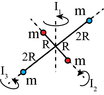
Fig. 13.17 An object of four masses: it can rotate around three different axes.

The object can rotate around three different axis. With each, a moment of inertia is associated.

Calculate the three moments of inertia and rank them from big to small. Around which axis is it easiest to set the object in rotation?

Exercise 13.2

Consider a thin disk (radius \(R\), mass \(M\), uniform density). The disc can spin about two different axes through its center. The first axis is perpendicular to the disc en goes through its center. It has an associated moment of inertia \(I_1\).

The second one is in the plane of the disc and goes over a diameter of the disc. It has associated moment of inertia \(I_2\)

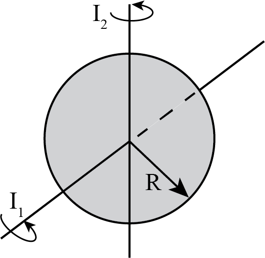
Fig. 13.18 A thin disc with two different axis of rotation.

Calculate the two moments of inertia.

Exercise 13.3

A cylinder (mass \(M\), radius \(R\), length \(L\)) can spin around its symmetry axis. Find the moment of inertia in case the density of the cylinder is a function of the distance to the symmetry axis:

\[\rho (r) = \rho_0 \left ( 1 - \frac{1}{2} \frac{r}{R} \right ) \]

The moment of inertia should be expressed in terms of \(M\), \(R\) and \(L\).

Exercise 13.4

You have a solid cylinder of mass \(M\) (with constant density) and a thin walled cylinder of the same mass \(M\), both rolling down an inclined slope of angle \(\alpha\). Which one will be down quicker? Compute their arrival times. If you need help, look here. For a good instruction video watch here, starting at 11:20.

The radius, \(R\), of the cylinders is not specified. Why is that not a problem?

Exercise 13.5

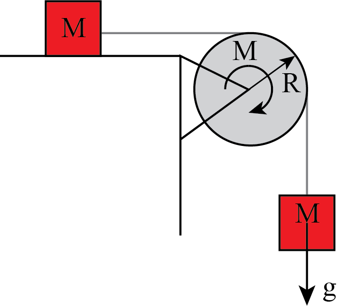
Fig. 13.19 Two masses and a pulley.

Consider the pulley-mass system in the figure above. A mass \(M\) can move frictionless over a table. The mass is attached via a massless, unstretchable rope over a disc (of constant density) of mass \(M as well and radius \)R\( to a second mass, also of mass \)M$. On the latter mass, gravity is working in the downward direction. The disc can rotate frictionless over a horizontal axis. The axis is fixed in space. The rope does not slip over the disc.

Find the velocity of the hanging mass as a function of time.

Exercise 13.6

A thin rod (length \(L\), mass \(M\), uniform density) is balancing at its tip. This is, however an unstable equilibrium position and the rod tumbles over. It does so without sliding, that is, the tip stays at the same position.

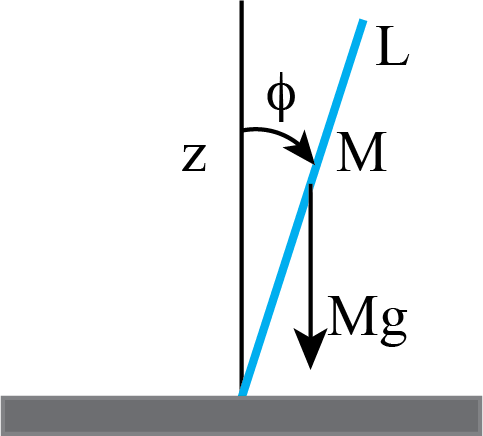
Fig. 13.20 Falling rod with fixed contact point.

With what velocity does the rod hit the floor?

Exercise 13.7

Same question as above, but now for the case the thin rod tumbles over while frictionless sliding with its tip over the surface.

With what velocity does the rod now hit the floor?

Exercise 13.8

In this exercise, we are going to look at a complex situation in which quite some of the concepts that we have studied need to be combined (if you can do this one by yourself, you are pretty much on your way mastering rigid bodies).

Study this exercise carefully: it contains a lot of the elements that we have discussed in a complex example. Try to keep an eye on the main ideas and not to get lost in all details that need to be calculated.

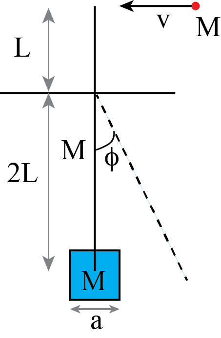
Fig. 13.21 A pendulum catching a point particle.

A pendulum made of a cube (mass \(M\), sides \(a\), uniform density) is at its center attached to a thin rod (length \(3L\), mass \(M\), uniform density). The rod is fixed to a horizontal axis around which it can rotate freely. A length \(L\) sticks out on one side of the axis, \(2L\) on the other. The pendulum is hanging in its equilibrium position.

A point particle of mass \(M\) is colliding at the free end of the rod with velocity \(v\). This velocity is horizontal. The collision is such, that the particle sticks to the tip of the rod.

1. Show that if \(v\) is sufficiently small, the pendulum will start to oscillate.

2. Find the oscillation frequency.

3. For what value of \(v\) will the pendulum exactly move upside down?

Before trying to solve this problem, first set up a procedure, i.e. describe the various steps to be taken.

13.13. Answers

Solution to Exercise 13.1

moment of inertia: $\( I \equiv \sum_s m_s r_s^2 \Rightarrow\)$

\[I_1 = 10mR^2\]

\[I_2 = 8mR^2\]

\[I_3 = 2mR^2\]

Thus \(I_1 \gt I_2 \gt I_3\); it is easiest to set the object in rotation around axis 3.

Solution to Exercise 13.2

moment of inertia: $\( I \equiv \sum_s m_s r_s^2 \Rightarrow\)$

\[I_1 = \frac{1}{2}MR^2\]

\[I_2 = \frac{1}{4}MR^2\]

Solution to Exercise 13.3

\[ I \equiv \sum_s m_sr_s^2 = \int r^2 dm \]

For the cylinder, we take as elements \(dm\) thin, concentric cylinders with length \(L\) and radius between \(r\) and \(r+dr\). The volume of such a thin cylinder is \(dV = L \cdot 2\pi r \cdot dr\) and thus its mass is \(dm = \rho (r) 2\pi L r dr\). If we plug this in, in the moment of inertia, we get:

\[\begin{split} \begin{split} I &= \int_0^R r^2 \rho_0 \left ( 1 - \frac{1}{2} \frac{r}{R} \right ) 2\pi L r dr \\ &= 2\pi \rho_0 R^4 L \int_0^1 (1 - \frac{1}{2}s ) s^3 ds \\ &= 2\pi \rho_0 R^4 L \left [ \frac{s^4}{4} - \frac{s^5}{10} \right ]_0^1 \\ &= 2\pi \rho_0 R^4 L \frac{3}{20} \end{split}\end{split}\]

Next, we need to find the relation between \(M\) and \(\rho_0\):

\[\begin{split} \begin{split} M &= \int \rho (r) dV \\ &= \int_0^R \rho_0 \left ( 1- \frac{1}{2} \frac{r}{R} \right ) 2\pi L r dr \\ &= 2\pi \rho_0 R^2 L \int_0^1 (1 - \frac{1}{2}s ) s ds \\ &= 2\pi \rho_0 R^2 L \left [ \frac{s^2}{2} - \frac{s^3}{6} \right ]_0^1 \\ &= \frac{2}{3} \pi \rho_0 R^2 L \end{split} \end{split}\]

Finally, we combine our expressions for \(I\) and \(M\):

\[ I = \frac{9}{20} MR^2 \]

Check: units = ok; our result is a smaller moment of inertia than a homogenous cylinder, this makes sense as due to the higher density closer to the axis, more mass is concentrate close to the rotation axis.

Solution to Exercise 13.4

thin walled: \(a_t = \frac{1}{2}g \sin \theta\)

massive: \(a_m = \frac{2}{3}g \sin \theta\)

Both roll a distance \(L\), starting from rest. Rolling time \(T=\sqrt{\frac{2L}{a}}\)

Thus, thin walled \(T_t = 2 \sqrt{\frac{L}{g \sin \theta}}\) and the massive one \(T_m = \sqrt{3} \sqrt{\frac{L}{g \sin \theta}}\). Hence the massive one is earlier at the end.

Solution to Exercise 13.5

We will use an energy consideration. We have three contributions to the kinetic energy:

\[ E_{kin} = \frac{1}{2} M v_1^2 + \frac{1}{2} I \omega^2 + \frac{1}{2}Mv_2^2\]

here, \(v_1\) is the velocity of the mass on the table and \(v_2\) that of the hanging mass. As the rope has a fixed length. The velocity of the two masses are the same (that is in magnitude, of course). We can thus drop the subscripts and call it \(v\). Moreover, due to the no-slipping of the rope we also have \(\omega = \frac{v}{R}\)

Using that for a homogenous disc \(I = \frac{1}{2}MR^2\), we can write the kinetic energy as

\[ E_{kin} = \frac{5}{4}Mv^2 \]

The potential energy is only coming from the hanging mass. If we define \(z=0\) when the hanging mass is pulled up against the disc, and take \(E_{pot} (z=0) = 0\), we have: \(E_{pot} = Mgz\). Thus the energy equation reads as

\[ \frac{5}{4}Mv^2 + Mgz = E_0\]

Differentiate with respect to time:

\[\frac{5}{2} Mv \dot{v} + Mgv = 0 \rightarrow \dot{v} = -\frac{2}{5}g \]

Let’s assume that at \(t=0\), \(z=0\) and \(v=0\) (the hanging mass is pulled al the way up to the disc and is released from rest), then

\[ v(t) = -\frac{2}{5}g t \]

Solution to Exercise 13.6

Before we start answering the question, we first need to think about the question itself: with what velocity does the rod hit the floor? Is there a single velocity? Do different parts not have different velocities?

Indeed, the rod rotates around its tip. The angular velocity of all parts will be the same, but the associated linear velocity varies from point to point. We will concentrate on the angular velocity.

The rod starts with only potential energy (and no kinetic energy):

\[E_{pot} = \int_0^L gz dm = \frac{1}{2}MgL\]

All this potential energy in converted to kinetic. When hitting the floor, the rod has an angular velocity \(\omega\).

\[E_{kin} = \frac{1}{2} I \omega^2\]

Moment of inertia for rotation around the tip:

\[I = \int_0^L z^2 \sigma dz = \frac{1}{3}ML^2 \]

Thus from conservation of energy we get:

\[0 + \frac{1}{2}MgL = \frac{1}{2} I \omega^2 + 0 \rightarrow \omega = \sqrt{3\frac{g}{L}}\]

Solution to Exercise 13.7

This case looks much like the previous exercise. However, in ex.(13.6) it was relatively straightforward to find the motion of the rod.

What do we now now? Since the tip in contact with the surface slides without friction, we have to conclude that at the point of contact there is no horizontal force from the surface on the tip. But there is a normal force at this tip.

Conclusion: during the falling down of the rod, there are only external forces acting on the rod in the vertical direction. Hence, it does not move horizontally. Or more precisely: its center of gravity falls vertically.

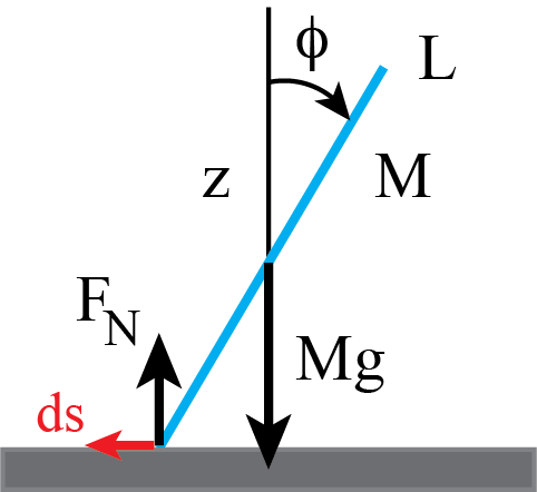
Fig. 13.22 Falling rod with sliding contact point.

Next, we need to deal with the question: does \(F_N\) perform work? In ex.(13.6), it doesn’t as the tip does not move in that case.

Here: \(d\vec{s}\) and \(\vec{F}_N\) are perpendicular and also here: no work is performed. Thus, we can analyse the system via conservation of kinetic plus potential energy.

kinetic energy

First, we realize that the center of gravity falls vertically down. On top of that the rod has to rotate. This rotating is due to the torque exerted by the normal force. The rotation is such, that the tip always makes contact with the floor. We see that the rod translates, so it has kinetic energy associated with the motion of its center of gravity. And it rotates around the center of gravity, giving rotational kinetic energy proportional to the moment of inertia for rotation around the center of gravity.

\[E_{kin} = \frac{1}{2} Mv^2 + \frac{1}{2}I\omega^2\]

\(v\) and \(\omega (=\dot{\phi})\) are coupled: the center of gravity is at a height \(z_{cg} = \frac{1}{2}L \cos \phi\) and thus:

\[ v = \frac{dz}{dt} = -\frac{1}{2}L \ sin \phi \,\, \omega \]

potential energy

We take the floor as \(E_{pot}=0\), then

\[E_{pot} = Mgz_{cg} = \frac{1}{2} MgL \cos \phi \]

Initially: \(v=0\), \(\omega = 0\), \(\phi = 0\) and the system has \(E_0= \frac{1}{2}MgL\).

In the final state: \(\phi = \frac{\pi}{2}\) and we want to calculate the velocity. The moment of inertia is (for rotation around an axis through the center of gravity):

\[I = \int_{-L/2}^{L/2} z^2 \sigma dz = \frac{1}{12}ML^2\]

If we combine all of the above, we get for initial to final

\[\begin{split} \begin{split} \frac{1}{2}M v^2 + \frac{1}{2}\frac{1}{12}ML^2 \left ( \frac{-2v}{L} \right)^2 + 0 = \frac{1}{2}MgL \rightarrow \\ v = \sqrt{\frac{3}{4}gL} \,\,\,\,\text{and} \,\,\,\, \omega = \sqrt{3g/L} \end{split} \end{split}\]

Solution to Exercise 13.8

We consider various steps:

1. “N2” for angular momentum or equivalently an energy consideration for the ‘swinging’ motion.

2. The collision: conservation of angular momentum with the origin taken at the pivot point (then the forces of the axis on the pendulum do not have torques).

3. Moment of inertia of pendulum prior to the collision.

4. Moment of inertia after collision

@1: energy will read something like \(\frac{1}{2}I\omega^2 + M_{tot}g z_{cg} = E_0\)

@2: the system has non-zero angular momentum prior to the collision. Thus after the collision we can compute the initial angular velocity from conservation of angular momentum.

@3+4: the system can be broken up in parts. For each part we can separately compute \(I\).

Calculation of moment of inertia

a) the cube

First for rotation around its center of gravity:

\[\begin{split} \begin{split} I_{s,cg} &= \int r^2 dm \\ &= \int_{-a/2}^{a/2}\int_{-a/2}^{a/2}\int_{-a/2}^{a/2} (x^2 + y^2 )\rho dxdydz \\ &= \rho \left [ z \right ]_{-a/2}^{a/2} \left ( \left [ \frac{x}{3}\right ]_{-a/2}^{a/2} \left [ y \right ]_{-a/2}^{a/2} + \left [ \frac{y}{3}\right ]_{-a/2}^{a/2} \left [ x \right ]_{-a/2}^{a/2} \right ) \\ &= \rho a \left ( \frac{a^3}{12} a + \frac{a^3}{12} a \right ) \\ &= \frac{1}{6}Ma^2 \end{split} \end{split}\]

Use Steiner’s theorem to find the moment of inertia for rotation around the pivotal point:

\[ I_s = M(2L)^2 + \frac{1}{6}Ma^2 = M \left ( 4L^2 + \frac{1}{6}a^2 \right )\]

b) the rod

\[\begin{split} \begin{split} I_r &= \int_{2L}^L z^2 \sigma dz \\ &= \sigma \left [ \frac{z^3}{3} \right ]_{-2L}^L \\ & = \sigma \frac{1}{3} ( L^3 - (-8L^3)) \\ &= ML^2 \end{split} \end{split}\]

c) the point particle (once attached to the rod)

\[I_p = ML^2\]

handling the collision

no external torques (friction at the axis has ‘no arm’, axis is assumed to be infinitely thin) \(\rightarrow\) angular momentum is conserved in the collision.

before: \(L_i = I_{pend, i} \underbrace{ \omega_i}_{=0} + \underbrace{MLv}_{incoming \; particle} \)

after: \(L_f = L_{pend} \, \omega_0 \)

Thus, with \(I_{pend} = M \left ( 4L^2 + \frac{1}{6}a^2 \right ) + ML^2 + ML^2 = 6ML^2 \left ( 1 + \frac{1}{36} \frac{a^2}{L^2} \right ) \) we get $\( \begin{split} \omega_0 &= \frac{ML}{ 6ML^2 \left ( 1 + \frac{1}{36} \frac{a^2}{L^2} \right )} v \\ &= \frac{1}{6 + \frac{1}{6} \frac{a^2}{L^2}} \frac{v}{L} \end{split} \)$

Energy consideration

After the collision, the pendulum rotates and thus has kinetic energy:

\[E_{kin} = \frac{1}{2} I_{pend} \omega^2\]

It has potential energy, that we find by computing the contribution of all individual masses making up the total system. Each elementary mass contribute \(dE_{pot} = m_i gz_i\)

\[\begin{split} \begin{split} E_{pot} &= \sum m_i gz_i \\ &= g \left ( \sum m_i \right ) \frac{\sum m_i z_i}{\sum m_i}\\ &= Mg z_{cg} \end{split} \end{split}\]

Thus, we see that we can also compute the center of gravity of the system we are dealing with. We may think of all mass concentrated in the center of gravity. This is handy, as for our swinging pendulum, it is as if (for the potential energy) all mass is located at the center of gravity and connected via a massless rod to the pivot point. Thus, if we have found the position of the center of gravity in our pendulum, we can use the same way of reasoning as with a simple pendulum: if the pendulum is displaced out of equilibrium, the center of gravity has just rotated over an angle \(\phi\) and the potential energy changes via the \(\cos \phi\).

First we will find the center of gravity and then, we will deal with the (potential) energy.

Center of Gravity A nice feature of the center of gravity is: it is a sum over parts, \(\sum m_i z_i\). We can chose how we split up this sum in parts and later add these parts to get the total sum. We will calculate \(\sum m_i z_i\) for the various parts. Note that we can do this for the pendulum hanging vertically downwards.

a) the cube

\[\begin{split} \begin{split} \sum_{cube} m_i z_i &= \int_{cube} z dm \\ &= \int_{-2L-a/2}^{-2L+a/2} z\, \rho a^2 dz \\ &= \rho a^2 \frac{1}{2} \left [ z^2 \right ]_{-2L-a/2}^{-2L+a/2} \\ &= \frac{1}{2} \rho a^2 \left ( L^2 - aL + \frac{a^2}{4} -L^2 -aL - \frac{a^2}{4} \right )\\ &= -\rho a^3 L \\ &= -M_{cube}L \end{split} \end{split}\]

b) the rod

\[\begin{split} \begin{split} \sum_{rod} m_i z_i &= \int_{rod} z dm \\ &= \int_{-2L}^L z\, \sigma dz \\ &= \sigma \frac{1}{2} \left [ z^2 \right ]_{-2L}^L \\ &= -\frac{1}{2}3\sigma L^2 \\ &= -\frac{1}{2}M_{rod}L \end{split} \end{split}\]

c) the point particle (once attached to the rod)

\[\sum_{p.p.} m_i z_i = M_{pp}L \]

Now we can compute the position of the center of gravity of the entire system:

\[\begin{split} \begin{split} z_{cg} &\equiv \frac{\sum m_i z_i}{\sum m_i} \\ &= \frac{-M_{cube}L - \frac{1}{2}M_{rod}L + M_{pp}L}{M_{cube} + M _{rod} + M_{pp}} \\ &= \frac{-ML -\frac{1}{2}ML + ML}{M+M+M} \\ &=-\frac{1}{6}L \end{split} \end{split}\]

Thus, the center of gravity is located at a distance \(L/6\) from the pivot point on the rod. Let’s call this \(L_{cg}\).

N2 for the pendulum

Finally, we can put all elements together and derive from our energy equation, N2:

\[\begin{split} \frac{1}{2} I_{pend} \omega^2 + 3Mg ( L_{cg} - L_{cg} \cos \phi ) = E_0 \end{split} \]

Take the time derivative:

\[ I_{pend} \ddot{\phi} + 3MgL_{cg} \sin \phi = 0 \]

with initial conditions:

\[ t= 0 \rightarrow \phi = 0, \,\,\, \omega = \frac{1}{6 + \frac{1}{6} \frac{a^2}{L^2}} \frac{v}{L} \]

We are now ready to answer the questions.

1. Indeed the pendulum will start to oscillate (provide the initial ‘kick is not so high that it will rotate rather than oscillate; we will find the restriction below). For large angles, it is not a harmonic oscillations, as the driving force is proportional to the \(\sin\) of \(\phi\), as is the case with the standard pendulum as well.

2. for small angles: \(\sin \phi \approx \phi\): $\(I_{pend} \ddot{\phi} + 3MgL_{cg} \phi = 0 \)$

Harmonic oscillator with frequency:

\[\begin{split} \begin{split} \Omega_0^2 &= \frac{3MgL_{cg}}{I_{pend}} \\ & = \frac{3Mg \frac{1}{6}L}{6ML^2 \left ( 1 + \frac{1}{36} \frac{a^2}{L^2} \right )} \\ &= \frac{1}{12 \left ( 1 + \frac{1}{36} \frac{a^2}{L^2} \right )}\frac{g}{L} \end{split} \end{split}\]

3. If the kinetic energy provided in the collision is sufficient, then the pendulum can rotate exactly 180\(^\circ\):

\[ \frac{1}{2}I_{pend} \omega_0^2 + 0 = 0 + 6MgL_{cg} \]

From this, we can calculate the necessary initial angular velocity right after the collision. We can put that in for the equation we found relating the incoming velocity to the angular velocity: \(\omega_0 = \frac{1}{6 + \frac{1}{6} \frac{a^2}{L^2}} \frac{v}{L}\).

This leads to

\[ v = \sqrt{12 \left ( 1 + \frac{1}{36} \frac{a^2}{L^2} \right ) gL} \]