
6. Angular Momentum, Torque & Central Forces#
6.1. Angular Momentum#
A useful quantity, especially but no exclusive, when it comes to rotation is the angular momentum, defined as
Angular Momentum
Angular momentum of a point particle is:
\( \vec{l} \equiv \vec{r} \times \vec{p} \)
Note that it is a cross product. Hence it is a vector itself. Further note that \(\vec{r} \times \vec{p} \neq \vec{p} \times \vec{r}\). The order matters! First \(\vec{r}\) then \(\vec{p}\). If you do it the other way around, you unwillingly have introduced a minus sign that should not be there.
Further note, that since \(\vec{l} \equiv \vec{r} \times \vec{p}\), \(\vec{l}\) is perpendicular to the plane formed by \(\vec{r}\) and \(\vec{p}\).
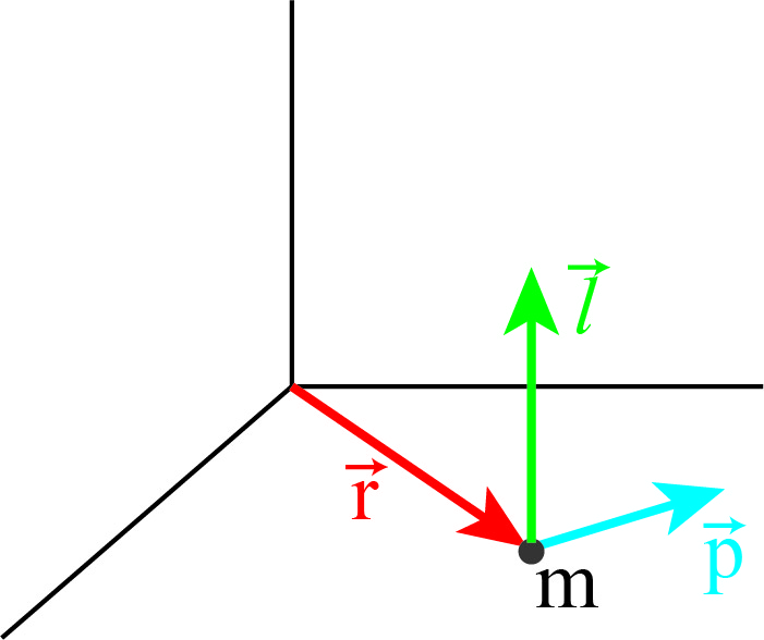
Fig. 6.1 Angular momentum of a particle at a certain position with a given momentum.#
6.1.1. Torque & Analogy to N2#
Angular momentum obeys a variation of Newton’s second law.
Thus, we find a general law for the angular momentum:
N2 for Angular Momentum
The rate of change of angular momentum is given by:
\( \frac{d \vec{l}}{dt} = \vec{r} \times \vec{F} \)
Again, note that the right hand side is a cross product, so the order does matter.
If we define the torque \(\vec{\Gamma}\) as the cross product of the particle position vector and the force acting on it
then we can write down an equation similar to N2 \((\dot{\vec{p}}=\vec{F})\) but now for angular momentum
where the force is replaced by the torque and the linear momentum by the angular momentum.
NB: Note that the torque and angular moment change if we choose a different origin as this changes the value of \(\vec{r}\).
Intermezzo: cross product
Here is some recap for the cross product. See also the wiki page.
Here \(\theta\) is the angle between \(\vec{a}\) and \(\vec{b}\), and \(\hat{n}\) is a unit vector normal to the plane spanned by \(\vec{a},\vec{b}\) with direction given by the right-hand rule.
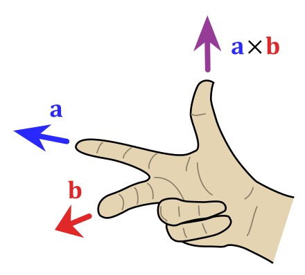
Fig. 6.2 Right hand rule for cross products. Adapted from Wikimedia Commons, licensed under CC-BY-SA 4.0.#
From the definition it is clear that \(\| \vec{a}\times\vec{b}\|\) is the area of the parallelogram spanned by \(\vec{a},\vec{b}\).
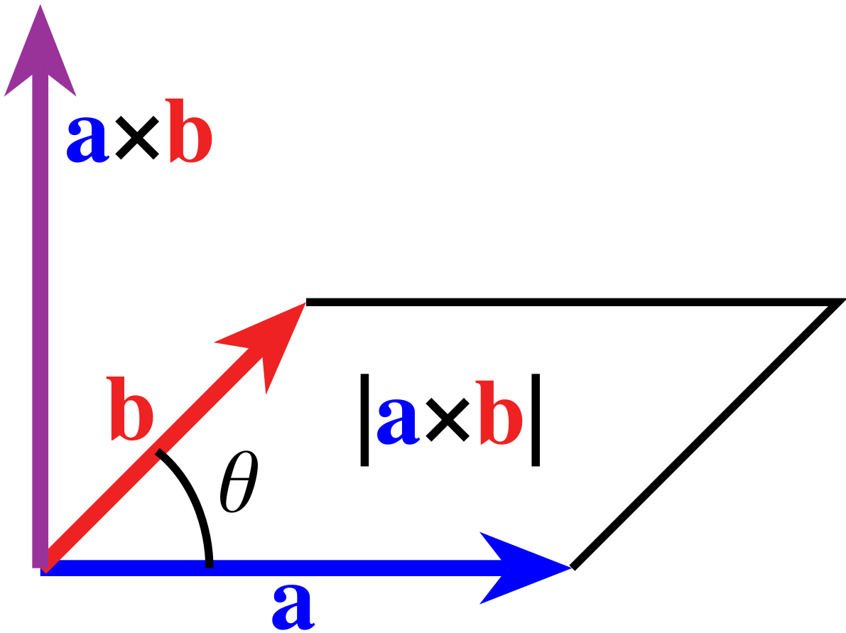
Fig. 6.3 Area of cross products. From Wikimedia Commons, public domain.#
The cross product is bilinear, anti commutative \((\vec{a}\times\vec{b} = -(\vec{b}\times\vec{a}))\) and distributive over addition.
The formula for computation in an orthonormal basis is
The formula can be derived from the cross product for orthonormal basis vectors, e.g. \(\hat{x},\hat{y},\hat{z}\)
Notice the cyclic structure of the equations.
It is a common mistake to identify angular momentum with rotational motion. That is not correct. A particle that travels in a straight line will, in general also have a non-zero angular momentum. See Fig. 6.4. Here we look at a free particle: there are no forces working on it. So it travels in a straight line, with constant momentum.
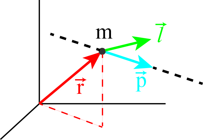
Fig. 6.4 Angular momentum of a free particle.#
However, the particle position does change over time. So: is its angular momentum constant or not?
That is easy to find out. We could take ‘N2’ for angular momentum:
Clearly, the angular momentum of a free particle is constant. Moreover, the momentum of a free particle is also constant. But what about the position vector: isn’t that changing over time and eventually becomes very, very long? Why does that not change \(\vec{r} \times \vec{p}\)?
Take a look at Fig. 6.5. We have chosen the \(xy\)-plane such that both \(\vec{r}\) and \(\vec{p}\) are in it. Furthermore, we have taken it such that \(\vec{p}\) is parallel to the \(x\)-axis.
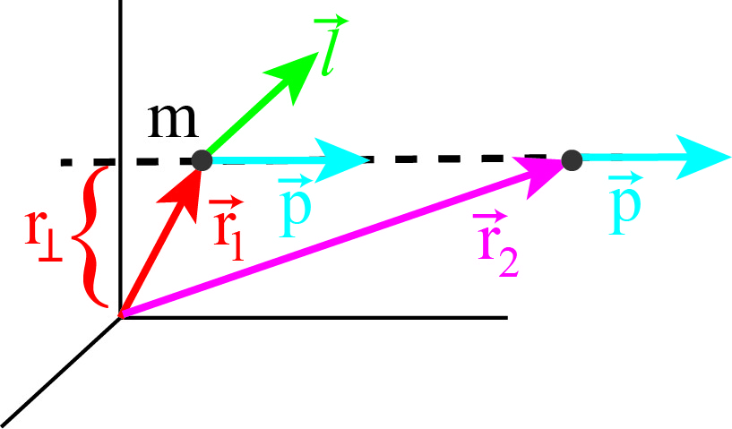
Fig. 6.5 Angular momentum of a free particle is constant.#
At some point in time, the particle is at position \(\vec{r}_1\). Its angular momentum is perpendicular to the \(xy\)-plane and has magnitude \(|| \vec{r}_1 \times \vec{p} || = r_\perp p\). Later in time it is at position \(\vec{r}_2\). Still, its angular momentum is perpendicular to the \(xy\)-plane and has magnitude \(|| \vec{r}_2 \times \vec{p} || = r_\perp p\), indeed identical to the earlier value. This shows that indeed the angular momentum of a free particle is constant.
6.2. Examples#
Example 6.1 Throwing a basketball
As seen in class: one person throws a basketball to another via a bounce on the ground, the basketball starts to spin after hitting the ground although initially it did not.
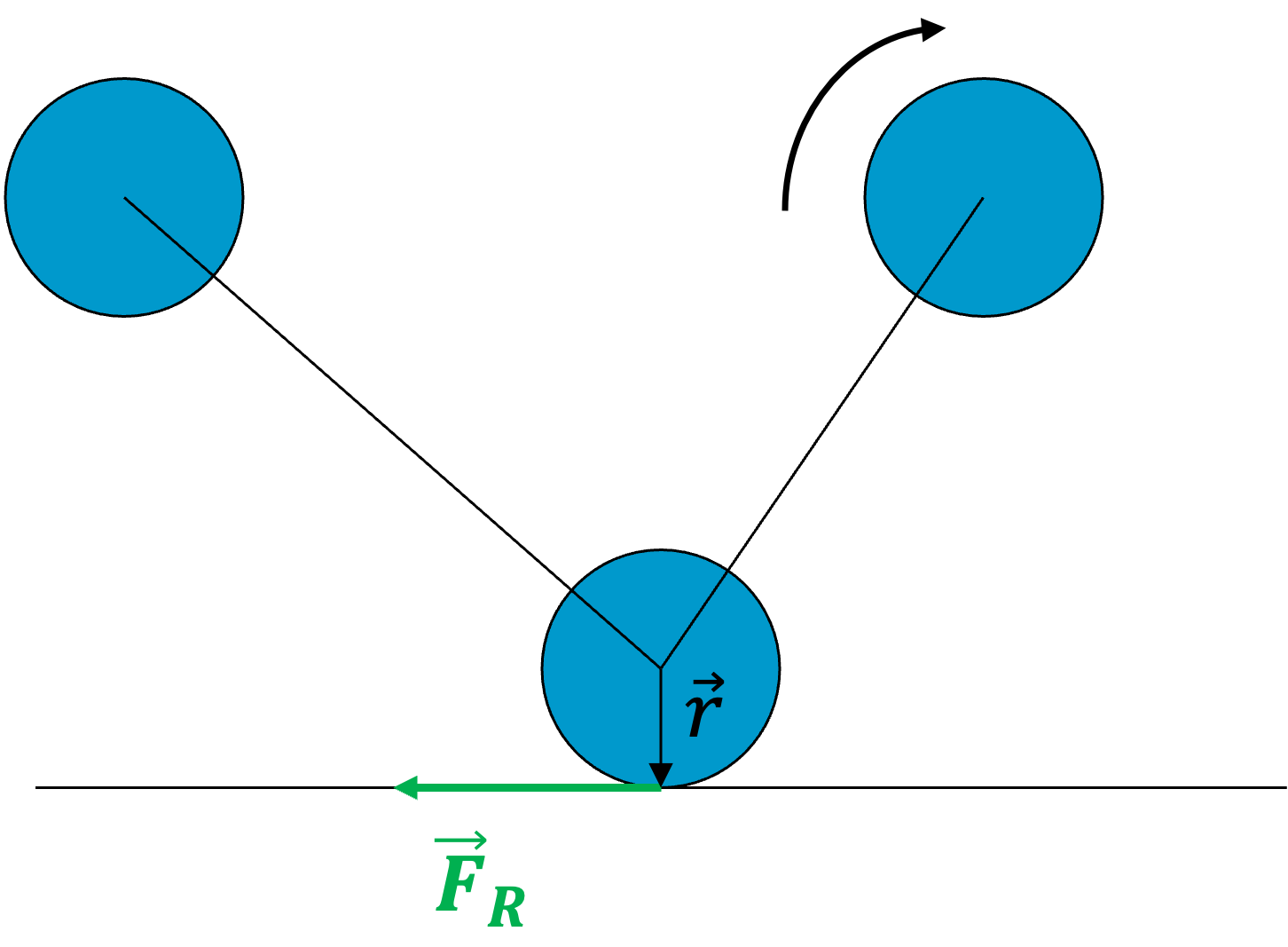
Fig. 6.6 Bouncing basketball#
When the ball hits the ground a friction force is acting on the ball. This force will apply a torque on the ball. The friction is directed opposite to the direction of motion. The arm \(\vec{r}\) from the center of the ball to where the force is acting, is downwards. Using the right-hand rule we find that the torque is pointing into the plane of the screen, and thus the rotation is clockwise (forwards spin).
The forwards momentum of the ball is reduced by the action of the force. The upwards components is just flipped by the bounce on the ground. Therefore the outgoing ball is bouncing up at a steeper angle than it is was incoming.
Example 6.2 Conservation of angular momentum & spinning wheel
As a demo, we have a student sitting on a chair that can rotate (swivel chair). The student is holding a bicycle wheel in horizontal position.
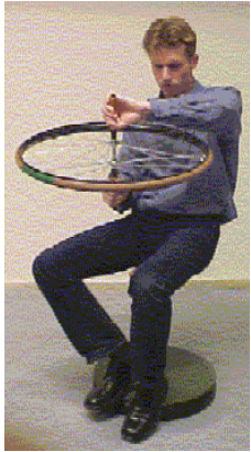
Fig. 6.7 Student with a rotating wheel#
Once the student starts to spin the wheel while sitting on the chair, the student will start to rotate in the opposite direction (with smaller angular velocity, lateron we will see why their speeds are different). Before the student starts spinning the wheel, the angular momentum of the student-wheel system is zero. But is has to remain zero, also after he spins the wheel: there is no net torque on the student-wheel system. To compensate for the angular momentum of the spinning wheel pointing up (counter clockwise rotation of the wheel), an angular momentum mpointing down (clockwise rotation of the student) of the same magnitude must occur.
6.3. Exercises#
Exercise 6.1
A point particle (mass \(m\)) is initially located at position \(P=(x_0,H,0)\). At \(t = 0\), it is released from rest and falls in a force field of constant acceleration \(\vec{a}=(0,-a,0)\) that acts on the mass (with \(a>0\)).
Analyze what happens to the angular momentum of \(m\).
Exercise 6.2
The same question, but now the particle has an initial velocity \(\vec{v} = (v_0 ,0,0)\).
Exercise 6.3
Similar situation: can you find an example of a falling object for which the angular momentum stays constant? Ignore friction with the air. Why is the latter statement important?
6.3.1. Answers#
Solution to Exercise 6.1

initial condition: \(t=0 \rightarrow \vec{v}=0 \rightarrow \vec{p}=0 \rightarrow \vec{p}=0 \rightarrow \vec{l}=0\)
Hence \(C=0\) and
i.e. the angular momentum points in the positive \(z\)-direction and linearly growth with time.
Solution to Exercise 6.2
The same analysis and sketch apply. The initial condition, however, is now different:
We still have:
But using the new initial condition we find:
Solution to Exercise 6.3

Cosider the case that the particle drops along the \(y\)-axis (i.e. compared to the previous exercises \(x_0=0\)). Now \(\vec{r}\) and \(\vec{F}\) are parallel and their cross product is zero.
Consequently:
What if there was air drag?
In that case, eventually the drag force will balance the downward accelerating force (if the particle can fall over e sufficient height). Once the two forces balance each other, the torque on the particle will be zero and thus from then on, the angular momentum of the particle will be constant.
6.4. Central Forces#
We have looked at a specific class of forces: the conservative ones. Here we will inspect a second class, that is very useful to identify: the central forces.
A force is called a central force if:
In words: a force is central of it points always into the direction of the origin or exactly in the opposite direction. The reason to identify this class is in the consequences it has for the angular momentum.
Suppose, a particle of mass \(m\) is subject to a central force. Then we can immediately infer that its angular momentum is a constant:
where we have use that \(\vec{r}\) and \(\hat{r}\) are always parallel so their cross-product is zero.
The above is rather trivial, but has a very important consequence: a particle that moves with a constant angular momentum (vector!) must move in a plane. It can not get out of that plane. Thus its motion is at maximum a 2-dimensional problem. We can always use a coordinate system, such that the motion of the particle is confined to only two of the three coordinates, e.g. we can choose our \(x,y\) plane such that the particle moves in it and thus always has \(z(t) = 0\).
Why is this so? Why does the fact that the angular momentum vector is a constant immediately imply that the particle motion is in a plane? The argumentation goes as follows.
Imagine a particle that moves under the influence of a central force. At some point in time it will have position \(\vec{r}_0\) and momentum \(\vec{p}_0\). Neither of them is constant. We will assume that \(\vec{r}_0\) and \(\vec{p}_0\) are not parallel ( in general they will not be). Thus they define a plane. Due to the cross-product \(\vec{l}_0 = \vec{r}_0 \times \vec{p}_0\) is perpendicular to this plane.
A little time later, say \(\Delta t\) later, both position and momentum will have changed. Since the force is central, the force is also in the plane defined by the initial position and momentum. Thus the change of momentum is in that plane as well: \(\vec{p} (t + \Delta t) = \vec{p} (t) + \vec{F} \Delta t\). The right hand side is completely in our plane. And thus, the new momentum is also in the plane. But that means that the velocity is also in the same plane. And thus the new position \(\vec{r} (t + \Delta t) = \vec{r}(t) + \frac{\vec{p}}{m} \Delta t\) must be in the same plane as well. We can repeat this argument for the next time and thus see, that both momentum and position can not get out of the plane.
6.5. Central forces: conservative or not?#
We can further restrict our class of central forces:
In the above, \(|\vec{F}(\vec{r})| = f(r)\), that is: the magnitude of the force only depends on the distance from the origin not on the direction. Rephrased: the force is spherically symmetric. If that is the case, the force is automatically conservative and a potential does exist. Both the concept of central forces and potential energy play a pivotal role in understanding the motion of celestial bodies, like our earth revolving the sun. We will take a look at the planetary motion as an example of dealing with central forces. It is, however, also an example in its own right. Using his new theory, Newton was able to prove that the motion of the earth around the sun is an ellipsoidal one. It helped changing the way we viewed the world from geo-centric to helio-centric.
6.5.1. Keppler’s Laws#
Before we embark at the problem of the earth moving under the influence of the sun’s gravity, we will go back in time a little bit.
Intermezzo: Tycho Brahe & Johannes Kepler
We find ourselves back in the Late Renaissance, that is around 1550-1600 AD. In Europe, the first signs of the scientific revolution can be found. Copernicus proposed his heliocentric view of the solar system. Galilei used his telescope to study the planets and found further evidence for the heliocentric idea. In Denmark, Tycho Brahe (1546-1601) made astronomical observations with data of unprecedented precision. He did so without the telescope as the first records of telescopes date back to around 1608 AD.

Fig. 6.8 left:Tycho Brahe (1546-1601) - right: Sophia Brahe (1559-1643). From Wikimedia Commons (L, R), public domain.#
Brahe initially studied law, but developed a keen interest in astronomy. He is heavily influenced by the solar eclipse of August 21st in 1560. The eclipse had been predicted via the theory of celestial motion at that time. However, the prediction was off by a day. This led Brahe to the conclusion that in order to advance celestial science, many more and much better observations were needed. He devoted much of his time in achieving this. One of his best assistants was his younger sister, Sophie.
On November 11th 1572, Brahe observed a bright, new star in the constellation Cassiopeia (it consists of five bright stars forming a M or W). That was another event that made him decide to spend his days gathering astronomical data. The current believe in those days was still that everything beyond the Moon was eternal, never changing. So, this new star, that all in a sudden appeared, must be closer to the earth than the Moon itself. Brahe set out to measure its daily parallax against the five stars of Cassiopeia. But he didn’t observe any parallax. Consequently, the new star’s position had to be farther out than the Moon and the other planets that did show daily parallax. Moreover, Brahe kept measuring for months and still found no parallax. That meant that this new star was even further out than the known planets that show no daily parallax but did so for periods of month. Brahe reached the conclusion that this new ‘thing’ thus could not be yet another planet, but that it was a star. Yet another nail to the coffin of the Aristotle view. Brahe wrote a small book about it, called De Nova Stella (published in 1573). He uses the term ‘nova’ for a new star. We see this back in our name for the phenomenon observed by Brahe: we call it a supernova. By now it is know that this new star, this supernova is some 7,500 light years away from us. Brahe was upset by those who denied the new findings. In his introduction of De Nova Stella he writes (given here in our modern words): “Oh coarse characters. Oh blind spectators of heaven”. The work and the booklet made his name in Europe as a leading scientist and astronomer.
in the winter of 1577-1578 a comet, known as the “Great Comet” appeared in the skies. It was observed by many all over the globe (from the Aztecs in the America’s via European researchers to the Arabic world, India all the way to Japan). Brahe made thousands of recordings, some simultaneously done in Denmark (close to Copenhagen) and Prague. That way, Brahe could establish that the comet was much beyond the Moon.
At the end of his life, Brahe moved to Prague to become the official imperial astronomer under the protection of Rudolf II, the Holy Roman Emperor. In the later part of his life, Brahe had Johannes Kepler as his assistant.
Kepler was 6 years old when the Great Comet appeared in the sky. He recorded in his writings that his mother had taken him to a high place to look at it. At the age of nine, he witnessed a lunar eclipse in which the Moon is in the Earth shadow, darkening it and turning it quite red. As a child he suffered from smallpox making his vision weak and limited his ability to use his hands. This made it difficult for him to make astronomical observations. It pushed him to mathematics. But there he was confronted with the Ptolemaic and the Copernican view on planetary motion. Kepler became a math professor at the Protestant Stiftsschüle in Graz. He wrote his ideas about the universe, following the thoughts of Copernicus in a book, that was read by Tycho Brahe. This brought him into contact with Brahe. In 1600 Kepler and his family moved to Prague as a consequence of political and religious oppression. He was appointed as assistant to Brahe and worked with Brahe on a new star catalogue and planetary tables. Brahe died unexpectedly on October 24th 1601. Two days later, Kepler was appointed as his successor.
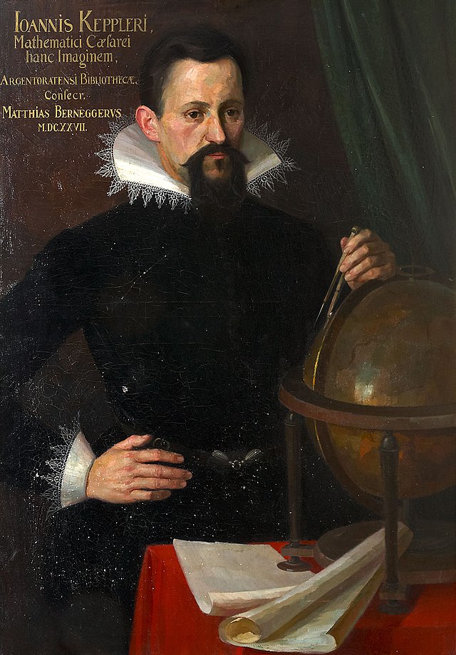
Fig. 6.9 Johannes Kepler (1571-1630). From Wikimedia Commons, public domain.#
Kepler worked on a heliocentric version of the universe and in the period 1609-1619 published his first two laws. With these he changed from trying circular orbits to other closed ones, to arrive at an elliptical one for Mars. That one was in very good agreement with the Brahe date, much better than had been achieved before. Kepler realized that the other planets might also be in elliptical orbits. In comparison with Copernicus he stated: the planetary orbits are not circles with epi-circles. Instead it are ellipses. Secondly, The sun is not at the center of the orbit, but in one of the focal points of the ellipse. Thirdly, the speed of a planet is not a constant.
Kepler’s work was not immediately recognized. On the contrary, Galilei completely ignored it and many critized Kepler for introducing physics into astronomy.
Kepler has formulated three laws that describe features of the orbits of the planets around the sun.
- The orbit of a planet is an ellipse with the Sun at one of the two focal points.
- A line segment joining a planet and the Sun sweeps out equal areas during equal intervals of time (Law of Equal Areas).
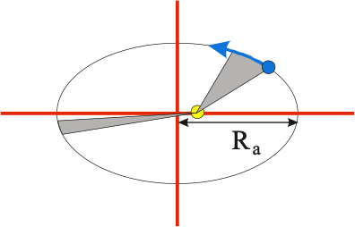
Fig. 6.10 Kepler’s 2nd Law of Equal Area.#
- The square of a planet's orbital period is proportional to the cube of the length of the semi-major axis of its orbit.
It is important to realize, that Kepler came to his laws by -what we would now call- curve fitting. That is, he was looking for a generic description of the orbits of planets that would match the Brahe data. He abandoned the Copernicus idea of circles with epi-circles with the sun in the center of the orbit. Instead he arrived at ellipses with the sun out of the center, in the focal point of the ellipse.
But, there was no scientific theory backing this up. It is purely ‘data-fitting’. Nevertheless, it is a major step forward in the thinking about our universe and solar system. It radically changed from the idea that the universe is ‘eternal’, that is for ever the same and build up of circles and spheres: the mathematical objects with highest symmetry showing how perfect the creation of the universe is.
Kepler had formulated his laws by 1619 AD. It would take another 60 years before Isaac Newton showed that these laws are actually imbedded in his first principle approach: all that is needed is Newton’s second law and his Gravitational Law. We will derive in the next section Kepler’s Laws from Newton’s laws.
6.6. Newton’s theory and Kepler’s Laws#
In order to derive Kepler’s laws from our Newtonian Mechanics, we will have to do some work. It starts with inspecting and classifying the force of gravity. Newton had formulated the Law of gravity: two objects of mass \(m_1\) and \(m_2\), respectively, exert a force on each other that is inversely proportional to the square of the distance between the two masses and is always attractive. In a mathematical equation, we can make this more precise:
In the figure below, the situation is sketched. We have chosen the origin somewhere and denote the position of the sun and the planet by \(\vec{r}_1\) and \(\vec{r}_2\). Gravity works along the vector \(\vec{r}_{12} = \vec{r}_2 - \vec{r}_1\). The corresponding unit vector is defined as \(\hat{r}_{12} = \frac{\vec{r}_{12}}{r_{12}}\).
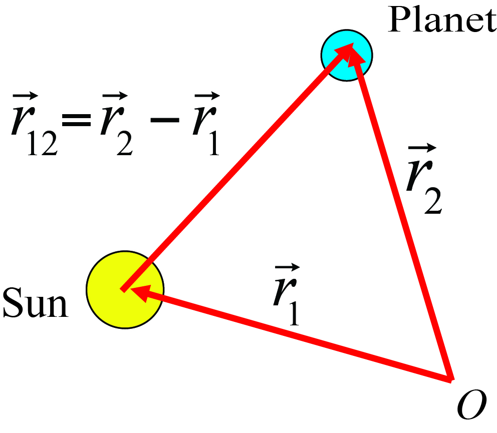
Fig. 6.11 The sun and a planet.#
Newton realized that he could make a very good approximation. Given that the mass of the sun is much bigger than that of a planet, the acceleration of the sun due to the gravitational force of the planet on the sun is much less than the acceleration of the planet due to the sun’s gravity. For this, we only need Newton’s 3rd law:
Hence
Newton concluded, that for all practical purposes, he could treat the sun as not moving. Next, he took the origin at the position of the sun. And from here on, we can ignore the sun and pretend that the planet feels a force given by
with \(M\) the mass of the sun and \(m\) that of the planet. \(r\) is now the distance from the planet to the origin and \(\hat{r}\) the unit vector pointing from the origin to the planet.
First observation The force is central!
First conclusion Then the angular momentum of the planet is conserved (it is a constant during the motion of the planet) and the motion is in a plane, i.e. we deal with a 2-dimensional problem!
Second Observation The force is of the form \(\vec{F}({\vec{r}}) = f(r) \hat{r}\)
Second conclusion Thus, we do know that a potential energy can be associated with it. It is a conservative force. This also implies that the mechanical energy of the planet, that is the sum of kinetic en potential energy, is a constant over time. In other words, since there is no frictional force, the motion can continue forever. This seems to be inline with our observation of the universe: the time scales are so large that friction must be small.
In order to progress and derive e.g. the Area Law, we need to further develop our mathematical toolbox. We will do that in the next section, where we concentrate on polar coordinates \((r, \phi )\).
6.7. Polar Coordinates#
We do know that the motion of the planet is confined to a plane. Hence we can use a Cartesian coordinate system, \((x, y)\) or a polar (also called cylindrical) one with coordinates \((r, \phi )\). These two are drawn in Fig. 6.12. Note that coordinates only get their full meaning if we provide unit vectors. For Cartesian coordinates, we are so used to these, that we don’t pay much attention to the unit vectors. But they are crucial.
If our planet is at time \(t\) at position \(\vec{r}\), we can give the coordinates: the planet is at \((x,y)\). What we actually mean is to say: the planet is at position \(\vec{r} = x \hat{x} + y\hat{y}\).
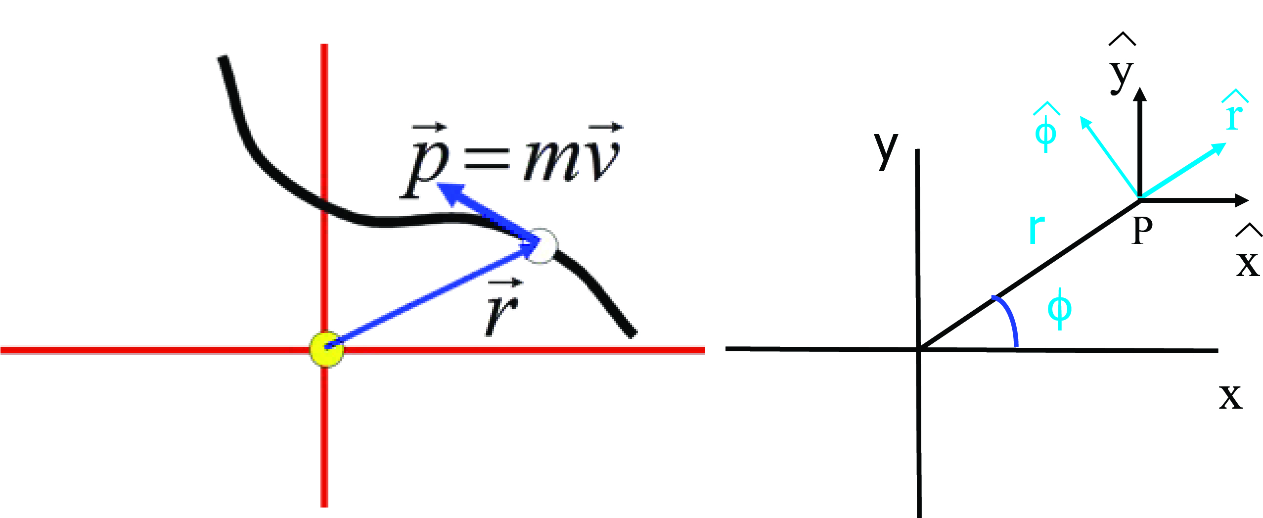
Fig. 6.12 Polar and Cartesian coordinates and unit vectors.#
However, we can equally well use Polar coordinates. With these we specify the distance \(r\) from the origin and give the direction to move into via the angle \(\phi\). We have to provide what \(\phi = 0\) means and we do that by saying that that is the \(x\)-axis. But actually, that is not needed. All we need to do is describe one direction in the 2-dimensional world as \(\phi = 0\). Nevertheless, it is convenient to call that direction the \(x\)-direction as we frequently switch between Polar and Cartesian coordinates.
How would, in our new Polar coordinate system that we are considering, point P be denoted?
First, we provide the coordinates: \((r, \phi )\). However, we need to represent the vector \(\vec{r}\). In essence this is a recipe that tells us how to ‘walk’ to get from the origin to the point P. In Cartesian coordinates this reads as \(\vec{r} = x\hat{x} + y\hat{y}\), which basically states: walk a distance \(x\) in the direction of \(\hat{x}\). Stop there and walk a distance \(y\) in the \(\hat{y}\) direction. In a Cartesian system this is trivial: \(\hat{x}\) and \(\hat{y}\) are always the same.
However, in Polar coordinates, this is somewhat more complex. Here our ‘walking recipe’ is: to get to \(\vec{r}\) walk a distance \(r\) in the \(\hat{r}\) direction. Simple, but strange: we seem to have no need for the second coordinate \(\phi\). We simply have \(\vec{r} = r \hat{r}\). But of course we need \(\phi\). \(r\) tells us how far we should walk, but it does not give the direction. That is provided by \(\hat{r}\) and to know the direction of \(\hat{r}\) we need to have \(\phi\).
This looks a bit puzzling at first sight. So, we better develop a formal set of relations between coordinates and unit vectors. This will allow us to ‘navigate’ between Polar and Cartesian coordinates and vice versa.
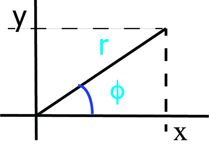
Fig. 6.13 Polar and Cartesian coordinates of the same point.#
From Fig. 6.13 we see that the coordinates are related to each other as:
or its inverse
The next step is to find relations that allow us to ‘translate’ the unit vector: \( ( \hat{r}, \hat{\phi } ) \leftrightarrow (\hat{x}, \hat{y} )\). We can do that using Fig. 6.14.
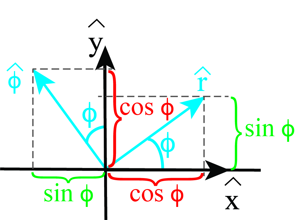
Fig. 6.14 Polar and Cartesian unit vectors.#
From this figure we can infer the recipe how to ‘go to’ position \(\hat{r}\). In Polar coordinates that is easy: walk one unit in the \(\hat{r}\) direction.
Cartesian we would do: walk \(\cos \phi\) in the \(\hat{x}\) direction and then \(\sin \phi \) in the \(\hat{y}\) direction. That we need to walk in the \(x\)-direction a distance of \(\cos \phi\) is easy to understand: that is exactly the length of the projection of \(\hat{r}\) on the \(x\)-axis. We can find confirmation in our rules for translating from \((r, \phi)\) to \((x, y)\) that we found above: take \(r=1\) (as the unit vector has length 1) and thus \(x = r \cos \phi = \cos \phi\).
We can write the above in an equation rather than in words: \( \hat{r} = \cos \phi \hat{x} + \sin \phi \hat{y} \)
We can also look at \(\hat{\phi }\). From Fig. 6.14 we see that we need to walk a distance \(\sin \phi\) in the negative \(x\)-direction and then \(\cos \phi \) in the \(y\)-direction. Thus: \( \hat{\phi} = -\sin \phi \hat{x} + \cos \phi \hat{y} \). We will write the two relations once more below.
If you progress further in physics and mathematics, you will learn that the above two equations signify a rotation over \(\phi\). And that is indeed how we started: rotation the ‘new, polar’ coordinate system over an angle \(\phi\) with respect to the ‘old, Cartesian’ one. Why is this useful to know? Well, that makes it almost trivial to find the inverse relation, that is the one expression \(\hat{x}\) and \(\hat{y}\) in terms of \(\hat{r}\) and \(\hat{\phi}\). All we need to do is realize that the inverse is a rotation over \(-\phi\): we have to rotate back. Thus, we see that the inverse is given by:
where we have used that \(\cos (-\phi ) = \cos \phi\) and \(\sin (-\phi ) = -\sin \phi\). If you don’t see the above immediately: don’t worry, it is not difficult to find the inverse relation. It is show below:
Subtract the two, last version from each other and you get:
or rewritten
which is identical to the result we had above.
Finding the expression for \(\hat{y}\) in a similar way is left as an exercise.
6.7.1. Velocity in Polar Coordinates#
Now that we have established the relations between coordinates and unit vectors, we can go one step further. In mechanics, we deal with velocity, momentum, acceleration etc. How do these relate to our new coordinates and unit vectors. At first sight it seems trivial: \(\vec{v} = \frac{d\vec{r}}{dt}\). So, we just need to do the differentiation in the new system.
6.7.1.1. Naive and wrong way#
Let’s first be naive and copy what we have been doing in Cartesian coordinates:
From which we get, that the coordinates of the velocity are: \((v_x, v_y )\).
So, we repeat the same but now using the Polar coordinates:
However, it is immediately clear that this must be wrong!!! After all, this would imply that the velocity is always in the direction of \(\hat{r}\) and that is simply not true. Take for instance the motion of a particle around a circle. Clearly, the distance from the origin is a constant for a circular motion. And thus \(\frac{dr}{dt} = 0\). According to our above ‘derivation’, that would mean that the velocity is zero!
So, what went wrong?
Actually, we might have been a bit hasty in deriving \(\vec{v}\) in the Cartesian system. The expression we found is correct, but the reasoning behind it might have missed an important point. Let’s go through the steps once more, but now with greater detail, not skipping steps. We start with the definition and the connection of the position to the Cartesian coordinates.
So far, so good. To proceed we have to use the product rule: \(\frac{d (f \cdot g)}{dt} = f \frac{dg}{dt} + g \frac{df}{dt}\). Thus, we write
We note that both \(\hat{x}\) and \(\hat{y}\) are unit vectors that are constant, i.e. their size doesn’t change (of course not: they have unit length) and their direction does not change (i.e. once we established the origin and both axis, the unit vectors are fixed and do not depend on time). We are so used to this, that we never think about \(\frac{d\hat{x}}{dt}\). It is zero anyhow. And thus, we can leave the two derivative of the unit vectors out of the equation and find what we had: \(\vec{v} = v_x \hat{x} + v_y \hat{y}\).
But for the Polar system, stuff is different! For different values of \(\phi\) the unit vectors \(\hat{r}\) and \(\hat{\phi}\) point in different directions. Thus, although their size is the same - always their lengths equals 1- their direction might change if we follow a particle from point to point. But this implies that \(\frac{d\hat{r}}{dt}\) and \(\frac{d\hat{\phi}}{dt}\) are not zero. How do we find the correct answers? Let’s start from the relation between the Polar unit vectors and the Cartesian ones.
We take the time-derivative:
Thus, we find that the change of the unit vector \(\hat{r}\) with time is in the direction of \(\hat{\phi}\). That of course makes sense: if \(\frac{d\hat{r}}{dt}\) had a component in the \(\hat{r}\) direction that would imply that its length would change. And that is of course not possible: it is a unit vector and will always have length 1.
It is also understandable that de rate of change of \(\hat{r}\) must scale with how quickly \(\phi\) changes with time. After all, changing position affects \(\hat{r}\) only if \(\phi\) changes. And the quicker \(\phi\) changes (that is, the larger \(\frac{d\phi }{dt}\)), the faster \(\hat{r}\) will change (thus, the bigger \(\frac{d\hat{r} }{dt}\)).
Now we have \(\frac{d\hat{r} }{dt}\), it is straightforward to copy the recipe to find \(\frac{d\hat{\phi} }{dt}\). Try to derive it yourself. You should find
Now, we can reconsider the velocity vector in Polar coordinates:
In summary, we have found for the Polar coordinate system:
Coordinate Transformation
and its inverse
Unit Vectors
and its inverse
Position Vector
Velocity Vector
Thus, we can represent the position by \((x,y)\) or \((r, \phi )\) and the velocity by \((v_x, v_y ) = \left ( \frac{dx}{dt}, \frac{dy}{dt} \right )\) or by \((v_r, v_\phi ) = \left ( \frac{dr}{dt}, r\frac{d\phi}{dt} \right )\).
6.8. Newton’s theory and Kepler’s Laws - part 2#
We have:
- The sun is replaced by a force field originating at the origin. This force field is a central force.
- Thus, the angular momentum is conserved.
- The orbit is in a plane: we deal with a 2-dimensional problem.
- The force is conserved: a potential exists.
Based on these, we will derive Kepler’s laws only using Newtonian Mechanics.
The first step is to calculate the angular momentum. Why? We know it is a constant as the force is central. Thus, during the motion of a planet around the sun, the angular momentum stays constant, giving a strong relation between the position and the momentum of the planet.
Angular momentum, \(\vec{l} \equiv \vec{r} \times \vec{p}\), can be represented in Cartesian as well as Polar coordinates. It is useful to use the latter. We will take our coordinate system such that the orbit of the planet is in the \(z=0\) plane.
Thus, we see that \(r\), that is the radial coordinate of the position of the planet and the angular velocity of the planet \(\dot{\phi}\) are related. The direction of the angular momentum is in the \(z\)-direction and it will stay that way as the vector angular momentum is a constant.
The magnitude of the angular momentum, \(l\), is constant too:
With this, we are surprisingly close to Kepler’s Equal Area Law. The argument goes as follows.
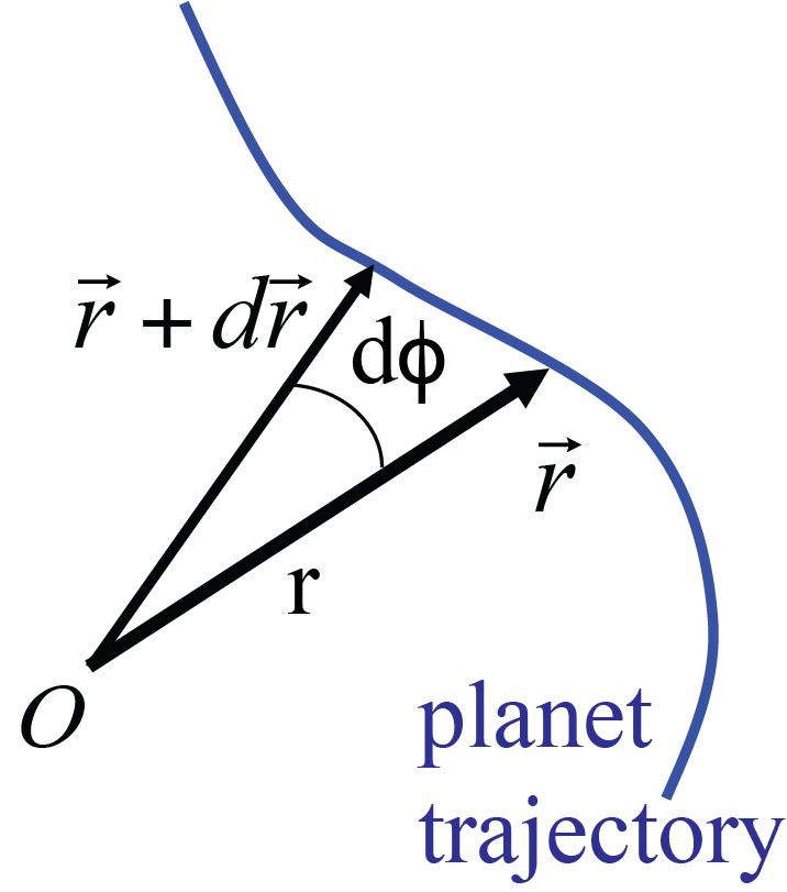
Fig. 6.15 Trajectory of a planet.#
Consider a planet moving through the \((r, \phi )\)-plane. It goes from its position \(\vec{r}\) at time \(t\) to \(\vec{r} + d\vec{r}\) at \(t+dt\), see Fig. 6.15. From the figure we get, that the area between the trajectory and the two positions is close to a triangular area. The smaller \(d\phi \) the better a triangle is to describe the area.
The area of the triangle is \(dA = \frac{1}{2} r \cdot rd\phi = \frac{1}{2}r^2 d\phi\).
This area is ‘swept’ in a time \(dt\). Thus the rate at which the planet sweeps through the area is
Now, we will eliminate \(\dot{\phi}\) using the angular momentum:
However, the above expression is constant, as both \(l\) and \(m\) are constant. In other words: in equal times, say \(\Delta t\), equal parts are swept: \(\frac{dA}{dt} = \frac{l}{2m} \rightarrow A(t) = A_0 + \frac{l}{2m}t \rightarrow \Delta A = \frac{l}{m} \Delta t\), which is a mathematical description of Kepler’s Equal Area Law!
6.8.1. Planets travel in ellipses#
To find the other two laws, we will have to work harder. We will start by an energy consideration. We know that our gravitational force is both central and conservative. Thus the sum of kinetic and potential energy is constant. Again, we will use Polar coordinates.
The kinetic energy is given by
The potential energy is found by solving \(V(r) = -\int_{r_{ref}}^r \vec{F}_g \cdot d\vec{r} \). We can plug in \(\vec{F}_g = - G \frac{mM}{r^2} \hat{r}\). Thus only the radial coordinate is of importance in the inner product in the integral. Furthermore, we will use as reference boundary: \(\infty\). Thus, the potential energy is:
Thus, energy conservation leads to:
As expected: we have an equation with two unknowns \((r(t), \phi (t))\). Once we solved the problem, we will thus have the coordinates of the planet’s trajectory as a function of time. However, we will not do that. Reason: it is complicated and we don’t need it! What we need is to find what kind of figure the trajectory is. And for that it is quite ok to find \(r\) as function of \(\phi\), that is, we will try to find \(r(\phi )\) and see whether or not that describes an ellipse.
Our first step is to bring the number of unknowns in the energy equation down from two to one. For that, we use again that the angular momentum is constant. This allows us to eliminate \(\dot{\phi}\):
We can interpret this in a different way: the second term originates from kinetic energy, but now looks like a potential energy. And that is exactly what we are going to do: treat it as a potential energy.
Now we can first inspect the global features of our energy equation. Notice that the gravity potential energy is an increasing function of the distance from the planet to the sun (located and fixed in the origin). This shows that the underlying force attractive is. The new part, coming from angular momentum, on the other hand is a decreasing function of distance. Thus, the related force is repelling.
We can make a drawing of the energy. See Fig. 6.16.
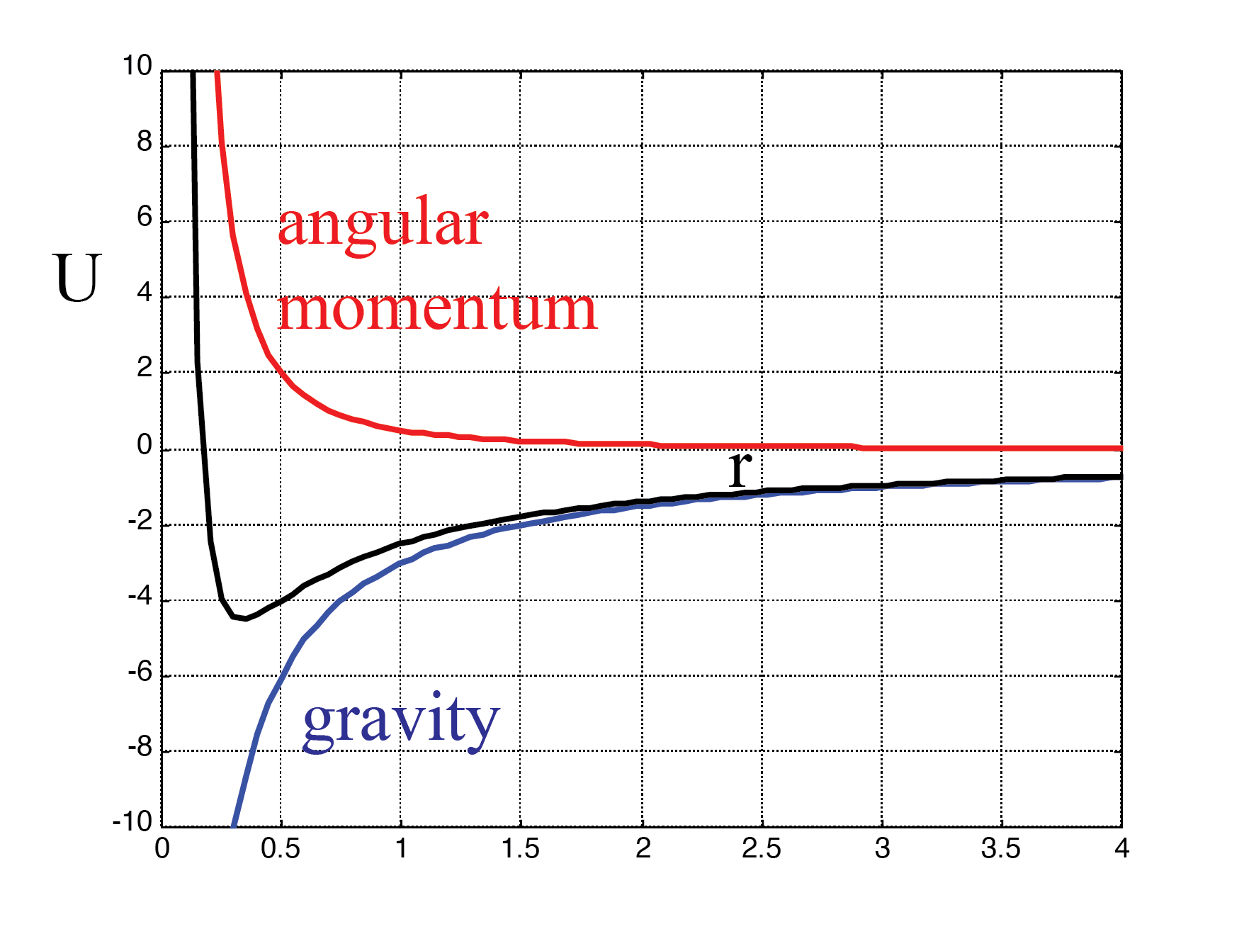
Fig. 6.16 Potential energy of a planet.#
The blue line is the potential energy of gravity. The red one stems from the kinetic energy associated with the angular velocity. The black line is the sum of the two, a kind of effective potential:
We see, that the energy can not be just any value: the kinetic energy of our quasi-one-dimensional particle (\(\frac{1}{2}m\dot{r}^2\)) can not be negative and the total potential energy has, according to Fig. 6.16 a clear minimum. The total energy can not be below this minimum. On the other hand: there is no maximum.
Case 1: \(U_{eff} = minimal\)
Suppose, we would prepare the system such that its total energy was equal to the minimum of the black line, i.e. of the total potential energy. Then, of course, via the arguments we have given above this is only possible if the kinetic energy is zero.
This implies that \(\dot{r} = 0\):
At first glance, this seems strange: \(\dot{r} = 0\) suggests that our particle doesn’t move, it has velocity zero. That would be strange: after all we are dealing here with a planet that is attracted via gravity towards the sun. How can it possible have zero velocity?
We are about to make a mistake: \(\dot{r} = 0\) doesn’t mean that the velocity is zero. It means that \(r(t) = const\). The planet still has an angular velocity: \(\dot{\phi} = \frac{l}{2mr^2} = const\) as in this particular case \(r = const\).
Thus, we conclude that for this case the planet moves at a constant distance around the sun at a constant angular velocity, that is: it moves in a circle at constant angular velocity.
Case 2: \(U_{eff, min} < E_{tot} < 0\)
Next, we consider a case where the total energy of the planet has a value between the minimum of the curve of the effective potential and 0. Call the value of the energy \(E_2\).
From Fig. 6.17 we see that the planet will now be confined to an area where the effective potential is either equal to or smaller than this particular value \(E_2\)
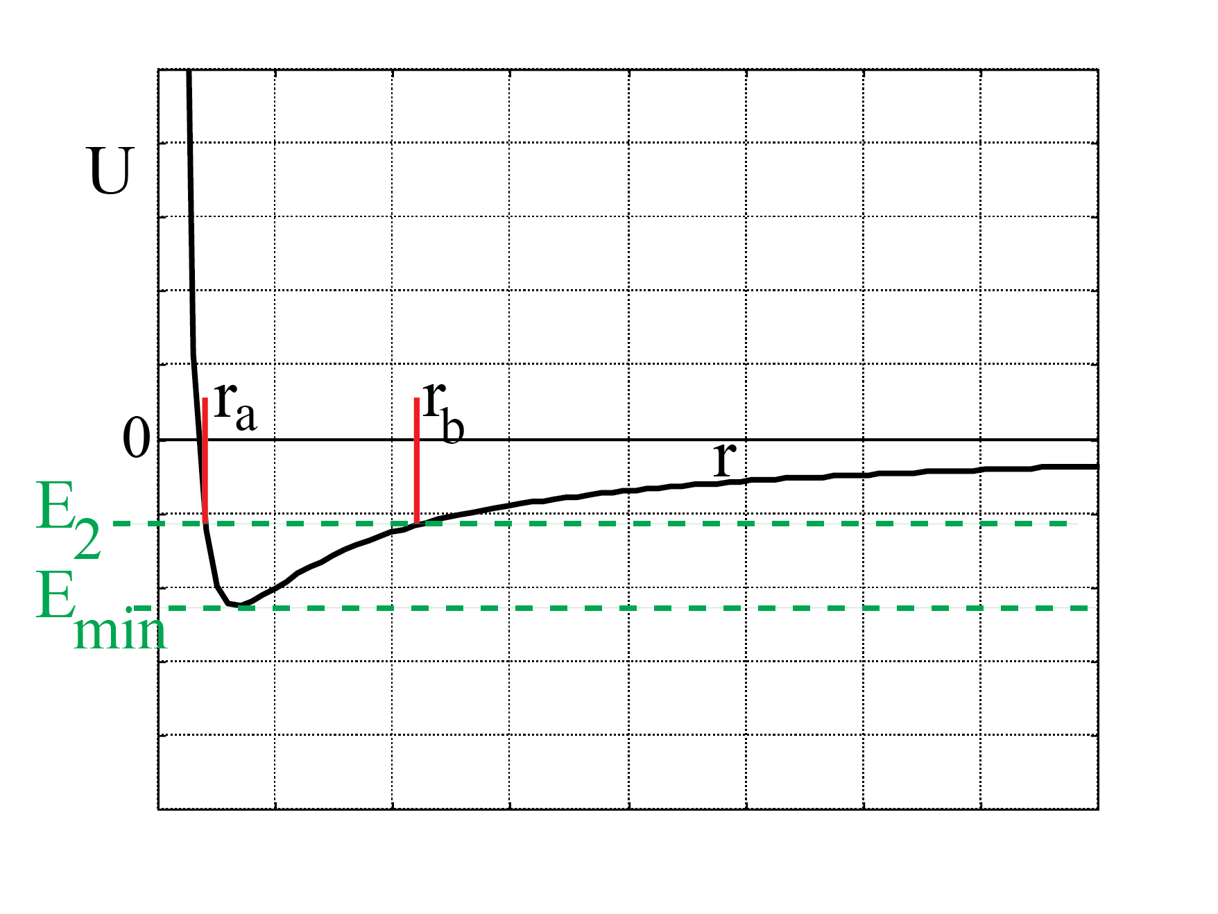
Fig. 6.17 Total energy between 0 and minimum of effective potential.#
Thus,the trajectory is confined between \(r=r_a\) and \(r=r_b\). At both these end points, the planet will have zero radial velocity: \(\dot{r}_a = \dot{r}_b = 0\). However, as before, the planet will still have angular momentum and thus still have a non-zero angular velocity. The planet will travel in the \((r,\phi )\)-plane between \(r=r_a\) and \(r=r_b\). How? We don’t know yet.
N.B. Do realize, that the angular velocity is for this case not a constant. We already have established that it is linked to the angular momentum (which is a constant) and the distance to the origin:
Thus, if the planet is closer to \(r_a\) it moves faster than close to \(r_b\). But it can not escape from \(r_a < r(t) < r_b\).
Case 3: \(E_{tot} \geq 0\)
Finally, we take the case that the total energy of the planet is positive (or zero), say a value of \(E_3\) in Fig. 6.18. Now we see that the planet can approach the sun, but not closer than a distance \(r=r_c\). The planet is attracted to the sun, but after reaching the closest distance \(r=r_c\) it will move away and eventually reach infinity. Again note: at \(r=r_c\), the planet does have a non-zero velocity.
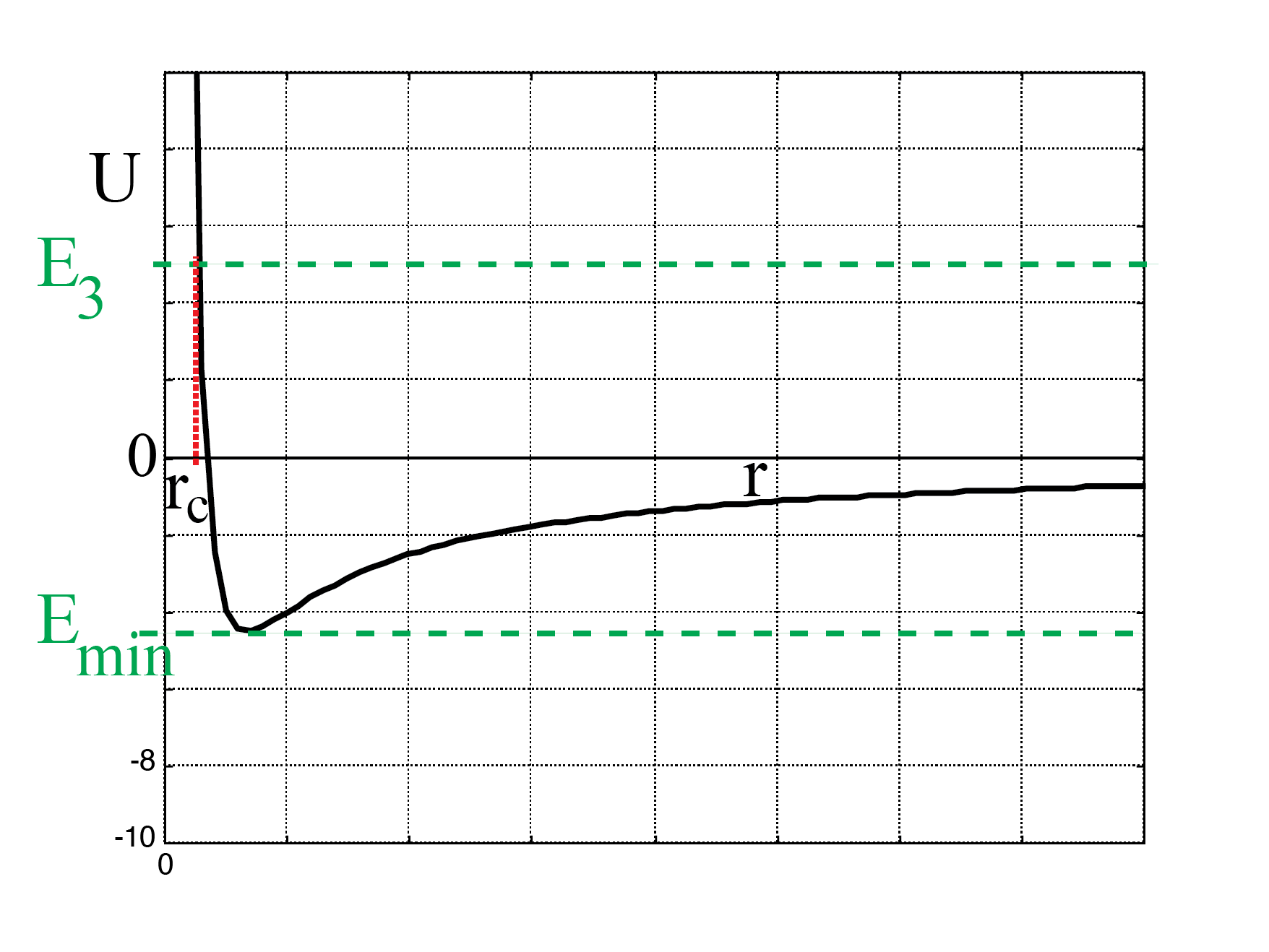
Fig. 6.18 Total energy larger than 0.#
6.8.1.1. Ellipsoidal orbits#
We are left with the task of showing that planets ‘circle’ the sun in an ellipse. From the above, we now know that this must mean that the total energy is smaller than zero: \(E<0\).
Below is the math of showing that the orbit is indeed an ellipse.
We are going to try and find \(r(\phi )\), rather than \(r(t)\) and \(\phi (t)\). Our starting point is
Notice that this is a differential equation for \(r(t)\). Its solution is constrained by:
It seems that this turns our problem back into a 2-dimensional one where we have to try to find \(r(t)\) and \(\phi (t)\). But we will not do so, as mentioned. Instead we will use the second equation to eliminate time derivatives from our problem.
First, we notice that in the energy equation we divide by \(r\) and \(r^2\). It will be easier to replace \(r\) by \(u \equiv \frac{1}{r}\)
Next, we use that \(r = r(\phi) = r(\phi (t))\). Thus for the time derivative of \(r\) we can write:
In \(\frac{dr}{d\phi}\) we replace \(r\) by \(\frac{1}{u}\):
Put the last two equation together:
We recognize the angular momentum in the third term:
Substitute this in the energy equation and we get:
You may not recognize this equation, but it has some similarities with \(\left ( \frac{df}{dx} \right )^2 + f^2 = 1\) which has as solution \(\sin\) and \(\cos\). To arrive at such an equation, we need to combine the second and third term (the two potentials) into one that is quadratic in the unknown function. This can be done in the following way:
Introduce the short-hand notation:
and we can write for the energy equation:
The second and the third term can be written ar:
Next, we introduce a new variable:
Obviously \(\frac{du}{d\phi } = \frac{1}{\alpha} \frac{dz}{d\phi }\). And we can, finally, cast our energy equation in a familiar form:
We place \(\alpha\) back and get:
So, finally, we have our energy equation in a form that is easy to solve:
with \(\phi_0\) an integration constant or re-phrased, the starting angle at the time we start to follow the planet on its trajectory.
We will now replace \(z\) by \(u\) and \(u\) by \(r\). That gives us the radial coordinate as function of the angle \(\phi\):
with
and
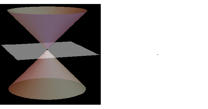
This type of curve in the \((r, \phi )\) plane is know as the conic sections. That is, they can be found by intersecting a cone with a plane.
Note that in the definition of \(e\), the total energy of the system plays a role. This energy can be negative (see Fig. 6.16). The minimum value of the effective potential energy is easily computed. It is \(U_{eff, min} = -\frac{1}{2} \frac{(GmM)^2m}{l^2}\) and is realized when the planet is at a distance \(r = \frac{l^2}{GMm^2}\). For this case we have \(e = 0\). This means that \(r(\phi ) = \alpha \), thus a constant: the planet is moving in a circle around the sun, as we already argued above.
For \(0 \leq e < 1 \) the orbit is an ellipse as Kepler already had postulated (for these values of \(e\) the orbit is a closed one).
For \(e=1\), the orbit is a parabola: the object will eventually move to infinity where it has exactly zero radial velocity.
Finally, for \(e > 1\) the trajectory is a hyperbola with the planet again moving to infinity.
We can change from Polar coordinates to Cartesian. This will give the following expression for the orbit in case of an ellipse:
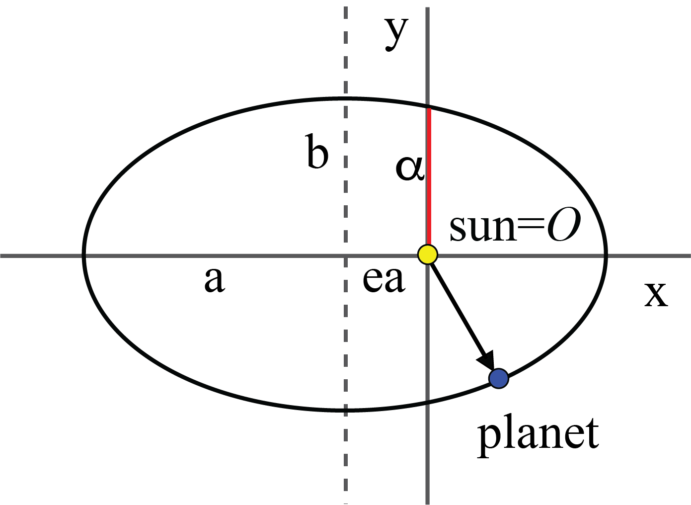
Fig. 6.20 Ellips in Cartesian coordinates.#
This is an ellipse with semi major and minor-axis \(a\) and \(b\), respectively. The center of the ellipse is located at \((-ea,0)\). Note that the sun is in the origin and that seen from the center of the ellipse, the origin is at one of the focal points of the ellipse. Consequently, the orbit is not symmetric as viewed from the sun. We notice this on earth: the summer and winter (when the sun is closest respectively furthest from the sun) are not symmetric, even if we take the tilted axis of the earth into account.
The half short and long axis are given by:
Conclusion: according to Newton’s laws of mechanics, combined with the Gravitation force proposed by Newton, planets must move in ellipses around their star.
This holds for our solar system, but for any other star with planets as well. Research has shown that there are hundreds of solar systems out in the universe with thousands of planets moving around their star. See e.g. https://exoplanets.nasa.gov/
6.8.2. Kepler 3#
We are left with proving Kepler’s third law:
Now that we know the orbit, this is not difficult. We concentrate on the motion during one lapse (one ‘year’). From Keppler’s 1st law we know that the area a planet sweeps out of its ellipse is given by
where \(C\) is an integration constant. Furthermore, this way of writing makes that the area swept keeps increasing: after one round along the ellipse, we simply keep counting.
However, we can easily back out what happens after exactly one round, or one ‘year’. The total area swept is then, of course, the area of the ellipse itself, that is: in one year (time \(T\)) the area swept is \(\pi a b\). Hence we conclude:
If we put back what we found for \(a\) and \(b\), we get
Thus, indeed Kepler was right. Moreover, we note that the constant is only depending on the mass of the sun. The same law will hold for other solar systems, but with a different constant.
In Fig. 6.21 Kepler’s third law is shown for our solar system. The red data points are based on the measured ‘year’ of each planet and the distance to the sun. The blue line is the prediction from Newton’s theory.
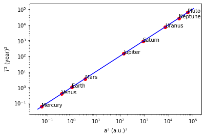
Fig. 6.21 Kepler 3 for our solar system.#
Haley’s comet
The planets aren’t the only objects that move around the sun. Several icy, rocky smaller objects are trapped in a closed orbit around the sun. These objects, comets from the Greek word for ‘long-haired star’, are left-overs from when our solar system was formed, some 4.6 billion years ago. There are many comets in our solar system. More than 4500 have been identified, but there are probably much more. Usually the orbit of a comet, if its is a closed one, has a high eccentricity (i.e. close to 1). Moreover, their orbital period may be very long.
One of the best visible comets is Haley’s comet. However, its orbital period is about 75 years. It last appeared in the inner parts of the Solar System in 1986. So, you will have to wait until mid-2061 to see it again.
Fig. 6.22 Trajectory of Haley’s comet. From Wikimedia Commons, licensed under CC-BY 4.0.#
6.9. The sun as a point mass#
In the above we assumed that the sun of mass \(M_{sun}=2\cdot 10^{30}\) kg with a radius of \(R_{sun}= 7\cdot 10^6\) km can be viewed as a point mass with the same mass for using Newton’s law of gravity. We just plugged in the mass, we did not bother about the mass distribution at all!
In fact this is allowed as long as the mass distribution is spherically symmetric as you will see below. We start from the gravitational (1D) potential \(V(x)=-G\frac{mm'}{x}\). For this potential holds \(\nabla V = -\vec{F}_g=-G \frac{mm'}{x^2}\hat{x}\). The derivation has a number of clever tricks to work out the integral and optimal choice of coordinates.
Moreover, the actual mass distribution of the sun does not matter, even if it would be non spherical. That is because the size of the sun is small compared to the distance to the earth. Any differences in the gravitational force are absolutely tiny because that distance is so large (radius of the sun is \(7\cdot 10^5\) km and the distance to the earth is \(>10^8\) km.
We consider a massive spherical shell with surface mass density \(\sigma\) (per unit area). Now compute the potential at some point \(P\) due to a part of the surface with coordinates \((r,\phi)\). P is at a distance \(x\) from the center of the shell and distance \(w\) from the part of the surface.
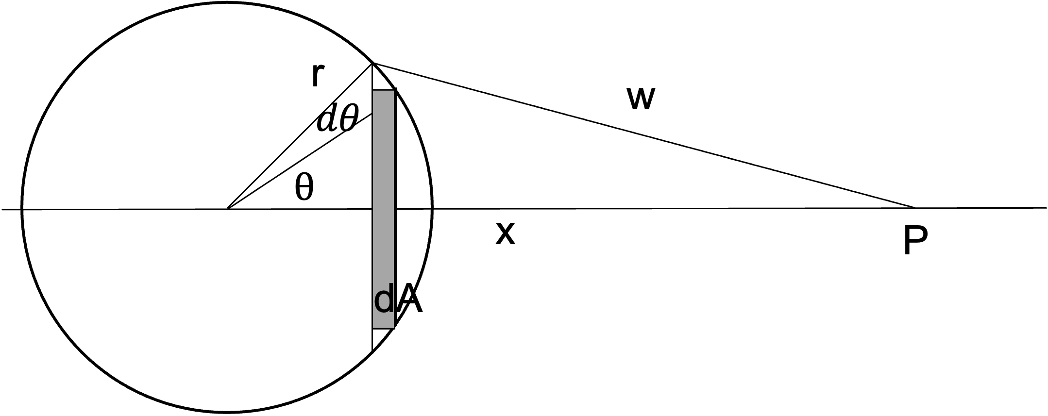
The potential is given as
with \(m'=\sigma dA\), \(dA=2\pi r \sin\theta\, rd\theta\) the revolution of the line element around \(2\pi\). If we additionally use the relation \(w^2=x^2+r^2-2xr\cos\theta\) to allow integration over \(w\) rather than \(\theta\), the differential is \(wdw = xr \sin\theta\,d\theta\). This is very similar to what we have in the nominator above, thus
If the point \(P\) is outside the shell, the angles varies \(\theta \in [0,\pi]\) or \(w\in[x-r,x+r]\) and we can calculate the potential
With the mass of the shell \(M=4\pi r^2\sigma\) we finally obtain
We see indeed that the mass distribution integrates out and we can deal with a point mass concentrated at the center of the shell. Hurray!
6.9.1. Gravity inside a shell#
The gravitational force inside a shell (hollow sphere) is zero - always - independent where inside of the shell you are. This result will pop up again in electrostatics where the electric force inside a charged spherical surface is zero. As the form of the gravitational and electric force are similar in their functional form \(\vec{F}(\vec{r})\propto r^{-2}\hat{r}\) this is not surprising. This a bit counter intuitive result is easy to see, if you apply Gauss theorem.
where \(\vec{f}\) is the gravitational \(\vec{f}=\frac{\vec{F}_g}{m}=-GM\frac{\hat{r}}{r^2}\) or electric field \(\vec{f}=\frac{\vec{F}_E}{q_0}= \frac{1}{4\pi\epsilon_0}\frac{q_1 \hat{r}}{r^2}\). The mass \(M\) (or charges \(q\)) is the sum of the mass inside the volume that the surface \(S\) encloses. If the surface does not enclose any mass (or charge), as is the case inside the shell, then the flux (\(\vec{f}\cdot dA\)) and field must be zero!
You can also integrate out the force as done here but that is quite some work.
6.10. Speed of the planets & dark matter#
Starting from Kepler 3, we can compute the orbital speed of a planet around the sun
Indeed if we measure the speed of the planets in the solar system this prediction holds, the velocity drops with the distance from the sun as \(\propto r^{-1/2}\) (see figure). As \(M\) we use the mass of the sun here.
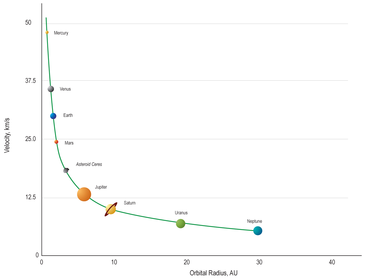
Fig. 6.23 From LibreTexts Physics, licensed under CC BY-NC-SA 4.0.#
The distance is measured in Astronomical Units [AU], the distance from the earth to the sun (about 8.3 light minutes). Note that the earth is moving with an unbelievable 30 km/s, that is \(10^5\) km/h! Do you notice any of that? We will use this motion later with the Michelson-Morley experiment.
If we plot the same speed versus distance curve not for the planets in our solar system, but for stars orbiting the center of our galaxy, the milky way, then the picture looks very different. The far away stars orbit at a much higher speed than expected and the form of the found curve does not match \(\propto r^{-1/2}\).
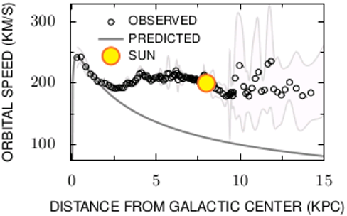
Fig. 6.24 From Wikimedia Commons, licensed under CC-SA 3.0.#
This mismatch is not understood to this day! The mass \(M\) here is calculated from the visible stars and the supermassive black holes at the center of the galaxy. But even if the mass is calculated wrongly, the shape of the dependency does not match. It turns out, this mismatch is observed in all galaxies! Apparently the law of gravity does not hold for large distances or there must be extra mass that increases the speed that we do not see. This mismatch has lead to the postulation of dark matter and an alternative formulation for the laws of gravity. This is the most disturbing problem in physics today; second is probably the interpretation of measurement in quantum mechanics (collapse of the wave function/Kopenhagen interpretation of Quantum Mechanics; multiverse theories).
The majority of all matter in the universe is believed to be dark. And we have no clue what it could be! Most scientist even think it must be non-baryonic, that is, other stuff than our well-known protons or neutrons. It remains most confusing.
The usual distance unit for distances in astronomy outside the solar system is not light years (ly), but parsec [pc], or kpc, or Mpc. One parsec is about 3.3 ly (or \(10^{13}\) km). Note: stars visible to the eye are typically not more than a few hundred parsec away. The milkyway is perfectly visible to the naked eye as a band/stripe of “milk” sprayed over the night sky. But you cannot see it anywhere close to Delft, there is much too much light from cities and greenhouses. Go to Scandinavia in the winter (“wintergatan”) or any place remote where there are few people. The reason you see a “band” in the night sky, is that the milky way is a spiral galaxy, sort of pancake shaped, and you see the band in the direction of the pancake.