2. Newton’s Laws

2.1. Newton’s Three Laws

Much of physics, in particular Classical Mechanics, rests on three laws that carry Newton’s name:

N1

If no force acts on an object, the object moves with constant velocity.

N2

If a (net) force acts on an object, the object will change its momentum according to:

\( \frac{d\vec{p}}{dt} = \vec{F} \)

N3

If object 1 exerts a force \( \vec{F}_{12} \) on object 2, then object 2 exerts a force \(\vec{F}_{21}\) equal in magnitude and opposite in direction on object 1:

\(\vec{F}_{21} = -\vec{F}_{12}\)

N1 has, in fact, been formulated by Galileo Galilei. Newton has, in his N2, build upon it: N1 is included in N2, after all:

if \(\vec{F} = 0\), then \(\frac{d\vec{p}}{dt} = 0 \rightarrow \vec{p} = const \rightarrow \vec{v} = cst\), provided \(m\) is a constant.

Most people know N2 as

\[ \vec{F} = m \vec{a} \]

For particles of constant mass, the two are equivalent: if \( m = const \), then \(\frac{d\vec{p}}{dt} = m\frac{d\vec{v}}{dt} = m\vec{a} \). Nevertheless, in many cases using the momentum representation is beneficial. The reason is, that momentum is one of the key quantities in physics. This is due to the underlying conservation law, that we will derive in a minute. Moreover, using momentum allows for a new interpretation of force: force is that quantity that -provided it is allowed to act for some time interval on an object- changes the momentum of that object. This can be formally written as:

\[ d\vec{p} = \vec{F} dt \leftrightarrow \Delta \vec{p} = \int \vec{F} dt \]

The later quantity \(\vec{I} \equiv \int \vec{F} dt\) is called the impulse.
Note for the Dutch students: momentum in English is impuls in Dutch; the English impulse is in Dutch ‘stoot’.

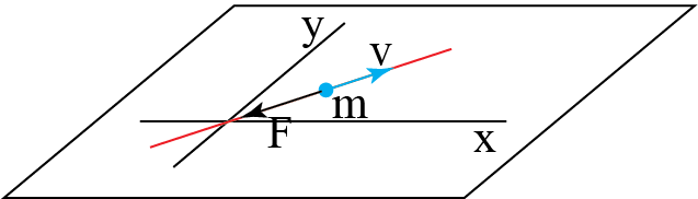
Example 2.1

Consider a point particle of mass m, moving at a velocity \( v_0 \) along the x-axis. At \( t=0 \) a constant force acts on the particle in the positive x-direction. The force lasts for a small time interval \( \Delta t \).
What is the velocity of the particle for \( t> \Delta t \) ?

Solution 2.1

First we make a sketch.

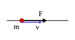
This is obviously a 1-dimensional problem. So, we can leave out the vector character of e.g. the force. We will use \( dp = F dt \):

\[ dp = Fdt \Rightarrow \Delta p = \int_0^{\Delta t} Fdt = F \Delta t \rightarrow \]

\[ p ( \Delta t) = p(0) + F \Delta t = mv_0 + F \Delta t \rightarrow\]

\[ v ( \Delta t ) = v_0 + \frac{F}{m} \Delta t \]

Note that this example could also be solved by N2 in the form of \(F = ma\). It is a matter of taste.

2.2. Time

In Newtons mechanics time does not have a preferential direction. That means, in the equations derived based on the three laws of Newton, we can replace \(t\) by \(-t\) and the motion will have different sign, but that is it. The path/orbit will be the same, but traversed in opposite direction. Also in special relativity this stays the same.

In daily life we experience a clear distinction between past, present and future. This difference is not present in this lecture at all. Only by the second of law thermodynamics the time axis obtains a direction, more about this in classes on Statistical Mechanics.

2.3. Note on vector notation

Note on vector notation

Position, velocity, momentum, force: they are all vectors. In physics we will use vectors a lot. It is important to use a proper notation to indicate that you are working with a vector. That can be done in various ways, all of which you will probably use at some point in time. We will take the position of a particle located at point P as an example.

2.3.1. Position vector

Position vector

We write the positionvector of the particle as \(\vec{r}\).
This vector is a ‘thing’, it exists in space independent of the coordinate system we use. All we need is an origin that defines the starting point of the vector and the point P, where the vector ends.
A coordinate system allows us to write a representation of the vector in terms of its coordinates. For instance, we could use the familiar Cartesian Coordinate system {x,y,z} and represent \(\vec{r}\) as a column.

\[\begin{split}\vec{r} \rightarrow \begin{pmatrix} x \\ y \\ z \end{pmatrix} \end{split}\]

Alternatively, we could use unit vectors in the x, y and z-direction. These vectors have unit length and point in the x,y or z-direction, respectively. They are denoted in varies ways, depending on your taste. Here are 3 examples:

\[\begin{split} \begin{split} \hat{x},\;\; \hat{i}, &\;\;\vec{e}_x \\ \hat{y},\;\; \hat{j}, &\;\;\vec{e}_y \\ \hat{z},\;\; \hat{k}, &\;\;\vec{e}_z \end{split} \end{split}\]

With this notation, we can write the position vector \(\vec{r}\) as follows:

\[\begin{split} \begin{split} \vec{r} &= x \hat{x} \;+ y \hat{y} \;+ z \hat{z} \\ \vec{r} &= x \hat{i}\;\; + y \hat{j}\; + z \hat{k} \\ \vec{r} &= x \vec{e}_x + y \vec{e}_y + z \vec{e}_z \end{split} \end{split}\]

Note that these last three are completely equivalent: the difference is in how the unit vectors are named. Also note, that these three representations are all given in terms of vectors. That is important to realize: in contrast to the column notation, now all is written at a single line. But keep in mind: \(\hat{x}\) and \(\hat{y}\) are perpendicular vectors.

Furthermore, note that the column representation provides us with the coordinates of the vector. We leave out the unit vectors in this notation, but we understand that the column with the coordinates means that the vector itself is found via \(x\hat{x} + y\hat{y} + z\hat{z}\).

2.3.2. Differentiating a vector

Differentiating a vector

We often have to differentiate physical quantities: velocity is the derivative of position with respect to time; acceleration is the derivative of velocity with respect to time. But you will also come across differentiation with respect to position.
As an example, let’s take velocity:

\[\vec{v} \equiv \frac{d\vec{r}}{dt} \]

What does it mean? Differentiating is looking at the change of your ‘function’ when you go from a point, \(x\), to a neighboring point, \(x+ \Delta x\) with \(\Delta x\) as small as we can make it:

\[\frac{df}{dx} \equiv \lim_{\Delta x \to 0} \frac{f(x + \Delta x ) - f(x)}{\Delta x}\]

In 3 dimensions we will have that we go from point P, represented by \(\vec{r} = x\hat{x} + y\hat{y} + z\hat{z}\) to ‘the next point’ \(\vec{r} + d\vec{r}\). The small vector \(d\vec{r}\) is a small step forward in all three directions, that is a bit \(dx\) in the x-direction, a bit \(dy\) in the y-direction and a bit \(dz\) in the z-direction.
Consequently, we can write \(\vec{r} + d\vec{r}\) as

\[ \vec{r} + d\vec{r} = x\hat{x} + y\hat{y} + z\hat{z} + dx\hat{dx} + dy\hat{y} + dz\hat{z} \]

\[= (x+dx)\hat{x} + (y+dy)\hat{y} + (z+dz)\hat{z}\]

Now, we can take a look at each component of the position and define the velocity component as e.g. in the x-direction

\[v_x = \lim_{\Delta t \to 0} \frac{x(t + \Delta t ) - x(t)}{\Delta t} = \frac{dx}{dt}\]

Applying this to the 3-dimensional vector, we get

\[\begin{split}\begin{split} \vec{v} \equiv \frac{d\vec{r}}{dt} &= \frac{d}{dt} \left ( x\hat{x} + y\hat{y} + z\hat{z} \right ) \\ &=\frac{dx}{dt}\hat{x} + \frac{dy}{dt}\hat{y} + \frac{dz}{dt}\hat{z} \\ &= v_x \hat{x} + v_y \hat{y} + v_z \hat{z} \end{split}\end{split}\]

Note that in the above, we have used that according to the product rule:

\[\frac{d}{dt} (x\hat{x} ) = \frac{dx}{dt}\hat{x} + x\frac{d\hat{x}}{dt} = \frac{dx}{dt}\hat{x}\]

since \(\frac{d\hat{x}}{dt} = 0\), the unit vectors in a Cartesian system are constant. This may sound trivial: how could they change? They have always length 1 and they always point in the same direction. Trivial as this may be, we will come across unit vectors that are not constant as their direction may change. But we will worry about those examples later.

2.4. Exercises

Exercise 2.1

Consider a point particle of mass m, moving at a velocity \( v_0 \) along the x-axis. At \( t=0 \) a constant force acts on the particle in the negative x-direction. The force lasts for a small time interval \( \Delta t \).
What is the strength of the force, if it brings the particle exactly to a zero-velocity?
Start by making a drawing.

Exercise 2.2

A particle of mass \(m\) moves along the \(x\)-axis. At time \(t=0\) it is at the origin with velocity \(v_0\). For \(t>0\) the particle feels a constant force. This is a 1-dimensional problem.

1. Calculate the acceleration of the particle as a function of time.
2. Calculate the velocity of the particle as a function of time.
3. Calculate the position of the particle as a function of time.

Exercise 2.3

A particle of mass \(m\) moves along the \(x\)-axis. At time \(t=0\) it is at the origin with velocity \(v_0\). For \(t>0\) the particle is subject to a force \(F_0 \sin (2\pi f_0 t)\). This is a 1-dimensional problem.

1. Calculate the acceleration of the particle as a function of time.
2. Calculate the velocity of the particle as a function of time.
3. Calculate the position of the particle as a function of time.

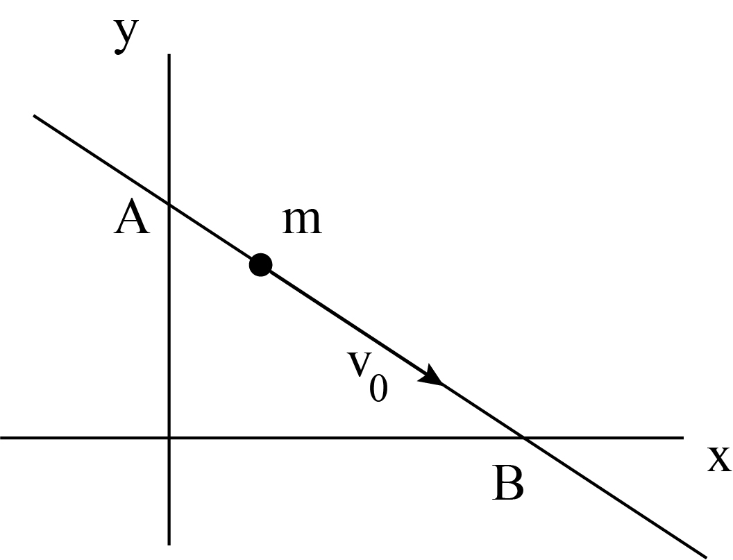
Exercise 2.4

A particle follows a straight path with a constant velocity. At \(t=0\) the particle is at point A with coordinate \(( 0, y_A)\), while at \(t = t_1\) it is at B with coordinate \((x_B, 0)\). The coordinates are given in a Cartesian system. The problem is 2-dimensional.

   a. Make a sketch.
   b. Find the position of the particle at arbitrary time \(0 < t < t_1\)
   c. Derive the velocity of the particle from its position as function of time.

Represent vectors in a Cartesian coordinate system using the unit vectors \(\hat{i}\) and \(\hat{j}.\)

Exercise 2.5

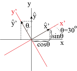
In Classical Mechanics we often use a coordinate system to describe motion of object. In this exercise, you will look at two Cartesian coordinate systems. System \(S\) has coordinates \((x, y)\) and corresponding unit vectors \(\hat{x}\) and \(\hat{y}\).
The second system, \(S'\), uses \((x', y')\) and corresponding unit vectors. The \(x'\)-axis makes an angle of \(30^\circ\) with the \(x\)-axis (measured counter-clockwise).
   a. Make a sketch.
   b. Determine the relations between \(\hat{x}'\) and \(\hat{x}, \hat{y}\) as well as between \(\hat{y}'\) and \(\hat{x}, \hat{y}\)
An object has, according to \(S\), a velocity of \(\vec{v} = 3 \hat{x} + 5 \hat{y}\).
   c. Determine the velocity according to \(S'\).

Exercise 2.6

According to your observations, a particle is located at position (1,0) (you use a Cartesian coordinate system). The particle has no velocity and no forces are acting on it.
Another observer, \(S'\), uses a Cartesian coordinate system described by \((x', y')\). You notice that her unit vectors rotate at a constant speed compared to your unit vectors:

\[\hat{x}' = \cos(2\pi f t ) \hat{x} + \sin(2\pi f t ) \hat{y}\]

\[\hat{y}' = -\sin(2\pi f t ) \hat{x} + \cos(2\pi f t ) \hat{y}\]

   a. Find the position of the particle according to the other observer, \(S'\).
   b. Calculate the velocity of the particle according to \(S'\).

Exercise 2.7

A particle of mass \(m\) moves at a constant velocity \(v_0\) over a frictionless table. The direction it is moving in, is at \(45^\circ\) with the positive \(x\)-axis. At some point in time, the particle experiences a force \(\vec{F} = -b \vec{v}\) with \(b>0\).
We call this time \(t=0\) and take the position of the particle at that time as our origin.
   a. Make a sketch.
   b. Determine whether this problem can be analyzed as a 1D problem or that a 2D approach is required.
   c. Set up N2 in the form \(m\frac{d\vec{v}}{dt} = \vec{F}\)
   d. Solve N2 and find the velocity of the particle as a function of time.
   e. What happens to the particle for large \(t\)?

2.5. Answers

Solution to Exercise 2.1

  \(\vec{F} = -\frac{m v_0}{\Delta t} \hat{x}\)

Solution to Exercise 2.2

1. \(a = \frac{F}{m}\) is constant

2. \(v(t) = v_0 + \frac{F}{m}t\)

3. \(x(t) = v_0 t + \frac{1}{2}\frac{F}{m}t^2\)

Solution to Exercise 2.3

1. \(a = \frac{F}{m} = \frac{F_0}{m} \sin (2\pi f_0 t) \) is not constant

2. \(v(t) = v_0 + \frac{F_0}{2 \pi f_0 m} \left ( 1 - \cos (2\pi f_0 t ) \right )\)

3. \(x(t) = v_0 t + \frac{F_0}{2 \pi f_0 m} \left ( t - \frac{1}{2\pi f_0 m}\sin (2\pi f_0 t ) \right )\)

Solution to Exercise 2.4

   a.

   b. Particle moves at constant velocity, thus its path is a straight line:

\[\vec{r}(t) = \vec{r}_0 + \vec{v}_0 t = x_0 \hat{i} + y_0 \hat{j} + v_{0x} t \hat{i} + v_{0y} t \hat{j}\]

At \(t=0: \vec{r}(0) = 0\hat{i} + y_A\hat(j) \rightarrow \vec{r}(0) = \vec{r}_0 = 0\hat{i} + y_A\hat{j} \rightarrow x_0 = 0 \text{ and } y_0 = y_A \)

At \(t=t_1: \vec{r}(t_1) = x_B\hat{i} + 0\hat(j) \rightarrow \vec{r}(t_1) = \vec{r}_0 +\vec{v}_0 t_1 = (0 + v_{0x}t_1 )\hat{i} + (y_A + v_{0y}t_1 ) \hat{j} \rightarrow v_{0x} = \frac{x_B}{t_1} \text{ and } v_{0y} = -\frac{y_A}{t_1} \)

   c. Thus, we find \(\vec{v} = \frac{x_B}{t_1} \hat{i} -\frac{y_A}{t_1}\hat{j} \)

Solution to Exercise 2.5

   a.

   b.

\[\begin{split} \begin{split} \hat{x}' = \cos \theta \hat{x} + \sin \theta \hat{y} = \frac{1}{2}\sqrt{3}\hat{x} + \frac{1}{2} \hat{y}\\ \hat{y}' = -\sin \theta \hat{x} + \cos \theta \hat{y} = -\frac{1}{2} \hat{x} + \frac{1}{2}\sqrt{3} \hat{y}\end{split}\end{split}\]

   c. Invert:

\[\begin{split} \begin{split} \hat{x} = \cos \theta \hat{x}' - \sin \theta \hat{y}' = \frac{1}{2}\sqrt{3}\hat{x}' - \frac{1}{2} \hat{y}'\\ \hat{y} = \sin \theta \hat{x}' + \cos \theta \hat{y}' = \frac{1}{2} \hat{x}' + \frac{1}{2}\sqrt{3} \hat{y}' \end{split}\end{split}\]

   velocity:

\[\begin{split}\begin{split} \vec{v} &= v_x \hat{x} + v_y \hat{y} \\ &= v_x \left ( \cos \theta \hat{x}' - \sin \theta \hat{y}' \right ) +v_y \left ( \sin \theta \hat{x}' + \cos \theta \hat{y}' \right ) \\ &= \left ( v_x \cos \theta + v_y \sin \theta \right ) \hat{x}' + \left ( -v_x \sin \theta + v_y \cos \theta \right ) \hat{y}' \end{split} \end{split}\]

    from which we find

\[ \vec{v} = \left ( \frac{3}{2}\sqrt{3} + \frac{5}{2} \right ) \hat{x}' + \left ( -\frac{3}{2} + \frac{5}{2}\sqrt{3} \right ) \hat{y}' \]

Solution to Exercise 2.6

   

\[\begin{split} \begin{split} \hat{x}' = \cos (2\pi ft) \hat{x} + \sin (2\pi ft) \hat{y}\\ \hat{y}' = -\sin (2\pi ft) \hat{x} + \cos (2\pi ft) \hat{y} \end{split}\end{split}\]

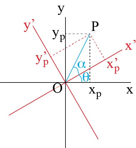
The unit vectors of \(S'\) rotate with a frequency \(f\) with respect to the unit vectors of \(S\). This means, that the coordinate system of \(S'\) rotates: the rotation angle is a function of time, i.e. \(\theta (t) = 2 \pi f t\)

From the figure we see, that the coordinates of a point P, \((x_p, y_p )\) according to \(S\), are related to those used by \(S'\), \( (x'_p, y'_p )\) via:

\[\begin{split} \begin{split} x_p = OP \cos ( \alpha + \theta ) = OP \left ( \cos \alpha \cos \theta - \sin \alpha \sin \theta \right) = x'_p \cos \theta - y'_p \sin \theta \\ y_p = OP \sin ( \alpha + \theta ) = OP \left ( \cos \alpha \sin \theta + \sin \alpha \cos \theta \right) = x'_p \sin \theta + y'_p \cos \theta \end{split} \end{split}\]

or written as the coordinate transformation:

\[\begin{split} \begin{split} x = x' \cos \theta - y' \sin \theta \\ y = x' \sin \theta + y' \cos \theta \end{split} \end{split}\]

with its inverse

\[\begin{split} \begin{split} x' = x \cos \theta + y \sin \theta \\ y' = -x \sin \theta + y \cos \theta \end{split} \end{split}\]

Note that in this case \(\theta = 2 \pi ft\), that is: it is a function of \(t\).

a) From the above relation we find that the point (1,0) in \(S\) will be denoted by \(S'\) as \((x'(t), y'(t)) = (\cos (2 \pi ft), -\sin ( 2\pi ft))\)

b) the velocity of the particle at point (1,0) in \(S\) is according to \(S\) of course zero: \(\frac{dx}{dt} = 0, \frac{dy}{dt} = 0\) \(S'\) will say:

\[\begin{split} \begin{split} x'(t) = \cos ( 2\pi ft) \rightarrow \frac{dx'}{dt} = -2 \pi f \sin (2\pi ft) \\ y'(t) = -\sin ( 2\pi ft) \rightarrow \frac{dy'}{dt} = 2 \pi f \cos (2\pi ft) \end{split} \end{split}\]

Solution to Exercise 2.7

a)

b) Since \(\vec{v}_0\) and \(\vec{F}\) are parallel, the particle will not deviate from the line x=y. Hence, we are dealing with a 1-dimensional problem. The original coordinate system, \((x,y)\), is not wrong: it is just not handy as it makes the problem look like 2D. Thus, we change our coordinate system, such that the new \(x\)-axis coincides with the original x=y line.

c) N2: \(m\frac{dv}{dt} = -b v\) with initial conditions: \(t= 0 \rightarrow x=0\) and \( t=0 \rightarrow v = v_0\)

d) \(\frac{dv}{dt} - \frac{b}{m} v = 0 \rightarrow v = A e^{-\frac{b}{m}t}\) initial condition: \(t= 0 \rightarrow v=v_0 \Rightarrow A = v_0\) Thus: \(v(t) = v_0 e^{-\frac{b}{m}t}\)

e) for \(t \rightarrow \infty: v \rightarrow 0\). The particle comes to rest and then, obviously, the friction force is zero.

2.5.1. A further note on notation: differentiation

A further note on notation: differentiation

Many physical phenomena are described by differential equations. That may be because a system evolves in time or because it changes from location to location. In our treatment of the principles of classical mechanics, we will use differentiation with respect to time a lot. The reason is obviously found in Newton’s \(2^{nd}\) law: \(F = ma\).

The acceleration \(a\) is the derivative of the velocity with respect to time; velocity in itself is the derivative of position with respect to time. Or when we use the equivalent formulation with momentum: \(\frac{dp}{dt} = F\). So, the change of momentum in time is due to forces. Again, we using differentiation, but now of momentum.

There are three common ways to denote differentiation. The first one is by ‘spelling it out’:

\[v = \frac{dx}{dt} \text{ and } a = \frac{dv}{dt} = \frac{d^2x}{dt^2}\]

Advantage: it is crystal clear what we are doing. Disadvantage: it is a rather lengthy way of writing. Newton introduced a different flavor: he used a dot above the quantity to indicate differentiation with respect to time. So,

\[v = \dot{x}, \text{ or } a = \dot{v} = \ddot{x}\]

Advantage: compact notation, keeping equations compact. Disadvantage: a dot is easily overlooked or disappears in the writing.

Finally, in math often the prime is used: \(\frac{df}{dx} = f'(x)\) or \(\frac{d^2f}{dx^2} = f"(x)\). Similar advantage and disadvantage as with the dot notation. Moreover, the prime is frequently used to denote a different observer, with a different coordinate system. We have seen the examples above. That is why many physicists don’t use the prime notation for differentiation.

2.6. Conservation of Momentum

From Newton’s 2\(^{\text{nd}}\) and 3\(^\text{rd}\) law we can easily derive the law of conservation of momentum.
Assume there are only two point-particle (i.e. particles with no size but with mass), that exert a force on each other. No other forces are present. From N2 we have:

\[\begin{split} \frac{d\vec{p}_1}{dt} = \vec{F}_{21} \\ \\ \frac{d\vec{p}_2}{dt} = \vec{F}_{12} \end{split}\]

From N3 we know:

\[ \vec{F}_{21} = -\vec{F}_{12} \]

And, thus by adding the two momentum equations we get:

\[\begin{split} \left. \begin{array}{ll} \frac{d\vec{p}_1}{dt} &= \vec{F}_{21} \\ \\ \frac{d\vec{p}_2}{dt} &= \vec{F}_{12} = -\vec{F}_{21} \end{array} \right \} \Rightarrow \end{split}\]

\[ \frac{d\vec{p}_1}{dt} + \frac{d\vec{p}_2}{dt} = 0 \rightarrow \frac{d}{dt} \left ( \vec{p}_1 + \vec{p}_2 \right ) = 0 \]

\[ \Rightarrow \vec{p}_1 + \vec{p}_2 = const ~\text{ i.e. does} \textit{ not } \text{depend on time} \]

Note the importance of the last conclusion: if objects interact via a mutual force then the total momentum of the objects can not change. No matter what the interaction is. It is easily extended to more interacting particles. The crux is that particles interact with one another via forces that obey N3. Thus for three interacting point particles we would have (with \( \vec{F}_{ij}\) the force from particle i felt by particle j):

\[\begin{split} \left. \begin{array}{ll} \frac{d\vec{p}_1}{dt} &= \vec{F}_{21} + \vec{F}_{31} \\ \\ \frac{d\vec{p}_2}{dt} &= \vec{F}_{12} + \vec{F}_{32}= -\vec{F}_{21} + \vec{F}_{32}\\ \\ \frac{d\vec{p}_3}{dt} &= \vec{F}_{13} + \vec{F}_{23}= -\vec{F}_{31} - \vec{F}_{32} \end{array} \right \} \end{split}\]

Sum these three equations:

\[\begin{split} \frac{d\vec{p}_1}{dt} + \frac{d\vec{p}_2}{dt} + \frac{d\vec{p}_3}{dt} = 0 \rightarrow \frac{d}{dt} \left ( \vec{p}_1 + \vec{p}_2 + \vec{p}_3 \right ) = 0 \\ \\ \Rightarrow \vec{p}_1 + \vec{p}_2 + \vec{p}_3 = const~\text{ i.e. does} \textit{ not } \text{depend on time} \end{split}\]

For a system of \(N\) particles, extension is straight forward.

2.6.1. Momentum example

The above theoretical concept is simple in its ideas: a particle changes its momentum whenever a force acts on it; momentum is conserved; action = - reaction. But it is incredible powerful and so generic, that finding when and how to use it is much less straight forward. The beauty of physics is its relatively small set of fundamental laws. The difficulty of physics is that these laws can be applied to almost anything. The trick is how to do that, how to start and get the machinery running. That can be very hard. Luckily there is a recipe to master it: it is called practice.

Example 2.2

A point particle (mass \(m\)) is dropped from rest at a height \(h\) above the ground. Only gravity acts on the particle with a constant acceleration \(g\) (=9.813 m/s\(^2\)).

1. Find the momentum when the particle hits the ground.
2. What would be the earth' velocity upon impact?

Solution 2.2

Let’s do this one together. We follow the standard approach of IDEA: Interpret (and make your sketch!), develop (think ‘model’), evaluate (solve your model) and assess (does it make any sense?).
First a sketch: draw what is needed, no more, no less.

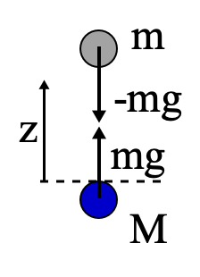
Actually this is half of the work, as when deciding what is needed we need to think what the problem really is. Above, is a sketch that could work. Both the object \(m\) and the earth (mass \(M\)) are drawn schematically. On each of them acts a force, where we know that on \(m\) standard gravity works. As a consequence of N3, a force equal in strength but opposite in direction acts on \(M\).
Why do we draw forces? Well, the question mentions ‘momentum the particle hits the ground’. Momentum and forces are coupled via N2.

We have drawn a z-coordinate: might be handy to remind us that this looks like a 1D problem (remember: momentum and force are both vectors).

As a first step, we ignore the motion of the earth. Argument? The magnitude of the ratio of the acceleration of earth over object is given by:

\[ \frac{a_e}{a_o} = \frac{| F_{o \rightarrow e} |/m_e}{| F_{e \rightarrow o} |/m_o} = \frac{m_o}{m_e} \]

here for the second equality we used N3.
For all practical purposes, the mass of the object is many orders of magnitude smaller than that of the earth. Hence, we can conclude that the acceleration of the earth is many orders of magnitude less than that of the object. The latter is of the order of \( g \), gravity’s acceleration constant at the earth. Thus, the acceleration of the earth is next to zero and we can safely assume our lab system, that is connected to the earth, can be treated as an inertial system with, for us, zero velocity.

The remainder is straightforward. Now we have an object, that moves under a constant force. So, its momentum will increase linearly in time:

\[ \frac{dp}{dt} = -mg \Rightarrow p(t) = m\underbrace{v_0}_{=0} - mgt = -mgt \]

From the momentum we can calculate the velocity and from the velocity the position:

\[ v = -gt \Rightarrow \frac{dz}{dt} = -gt \Rightarrow z(t) = \underbrace{z_0}_{=H} - \frac{1}{2}gt^2 = H - \frac{1}{2}gt^2 \]

Solve for \(z(T) = 0 \) and find \( T = \sqrt{\frac{2H}{g}} \). Substitute this into the relation for \( v \): \( v(T) = -\sqrt{2gH} \). As the earth-object system has conserved momentum, the velocity of the earth is to a good approximation:

\[ p_e + p_o = 0 \Rightarrow v_e = - \frac{m_o}{m_e} v_o = \frac{m_o}{m_e} \sqrt{2gH} \]

2.7. Forces & Inertia

Newton’s laws introduce the concept of force. Forces have distinct features:

• forces are vectors, that is, they have magnitude and direction;
• forces change the motion of an object: they change the velocity, i.e. they accelerate the object
  (2.1)\[\vec{a} = \frac{\vec{F}}{m} \leftrightarrow d\vec{v} = \vec{a}dt = \frac{\vec{F}dt}{m}\]

  or, equally true:

  they change the momentum of an object

  (2.2)\[\frac{d\vec{p}}{dt} = \vec{F} \leftrightarrow d\vec{p} = \vec{F}dt \]

Many physicists like the second bullet: forces change the momentum of an object, but for that they need time to act.

Momentum is a more fundamental concept in physics than acceleration: momentum is a conserved quantity; there is no law of conservation of acceleration. That is another reason why physicists prefer the second way of looking at forces.

2.7.1. Inertia

Inertia is denoted by the letter \( m \) for mass. And mass is that property of an object that characterizes its resistance to changing its velocity. Actually, we should have written something like \( m_i \), with subscript i denoting inertia.

Why? there is another property of objects, also called mass, that is part of Newton’s Gravitational Law.

Two bodies of mass \( m_1 \) and \( m_2 \) attract each other via the so-called gravitational force:

(2.3)\[\vec{F}_{12} = - G \frac{m_1 m_2}{r^2_{12}}\hat{r}_{12}\]

Here, we should have used a different symbol, rather than \( m \). Something like \( m_g \), as it is by no means obvious that the two ‘masses’ \( m_i \) and \( m_g \) refer to the same property. If you find that confusing: think about inertia and electric forces: you denote the property associated with electric forces by \( q \) and call it charge. We have no problem writing

\[\begin{split}\vec{F} = m \vec{a} \\ \vec{F}_C = \frac{1}{4\pi \epsilon_0} \frac{q Q}{r^2} \hat{r} \end{split}\]

We do not confuse \(q\) by \(m\) or vice versa. They are really different quantities: \(q\) tells us that the particle has a property we call ‘charge’ and that it will respond to other charges, either being attracted to or repelled from. How fast it will respond to this force of another charged particle depends on \(m\). If \(m\) is big, the particle will only get a small acceleration; the strength of the force does not depend on \(m\) at all. So far, so good. But what about \(m_g\)? That property of a particle that makes it being attracted to another particle with this same property, that we could have called ‘gravitational charge’. It is clearly different from ‘electrical charge’. But would it not have been logical that it was also different from the property inertial mass, \(m_i\)?

\[\begin{split}\vec{F} = m_i \vec{a} \\ \vec{F}_g = -G \frac{m_g M_g}{r^2} \hat{r} \end{split}\]

As far as we can tell (via experiments) \( m_i \) and \( m_g \) are the same. Actually, it was Einstein who postulated that the two are referring to the same property of an object: there is no difference.

2.7.1.1. Measuring mass or force

So far, we did not address how to measure force. Neither did we discuss how to measure mass. This is less trivial than it looks at first side. Obviously, force and mass are coupled via N2: \( F = m a \).

The acceleration can be measured when we have a ruler and a clock, i.e. once we have established how to measure distance and how to measure time intervals, we can measure position as a function of time and from that velocity and acceleration.

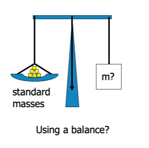
But how to find mass? We could agree upon a unit mass, an object that represents by definition 1kg. In fact we did. But that is only step one. The next question is: how do we compare an unknown mass to our standard. A first reaction might be: put them on a balance and see how many standard kilograms you need (including fractions of it) to balance the unknown mass. Sounds like a good idea, but is it? Unfortunately, the answer is not a ‘yes’.

As on second thought: the balance compares the pull of gravity. Hence, it ‘measures’ gravitational mass, rather than inertia. Luckily, Newton’s laws help. Suppose we let two objects, our standard mass and the unknown one, interact under their mutual interaction force. Every other force is excluded. Then, on account on N2 we have

\[\begin{split} \left. \begin{array}{ll} m_1 a_1 &= F_{21} \\ m_2 a_2 &= F_{12} = -F_{21} \end{array} \right \} \end{split}\]

where we used N3 for the last equality. Clearly, if we take the ratio of these two equations we get:

\[ \frac{m_1}{m_2} = \left | \frac{a_2}{a_1} \right | \]

irrespective of the strength or nature of the forces involved. We can measure acceleration and thus with this rule express the unknown mass in terms of our standard.

Note, we will not use this method to measure mass. We came to the conclusion that we can’t find any difference in the gravitational mass and the inertial mass. Hence, we can use scales and balances for all practical purposes. But the above shows, that we can safely work with inertial mass: we have the means to measure it and compare it to our standard kilogram.

Now that we know how to determine mass, we also have solved the problem of measuring force. We just measure the mass and the acceleration of an object and from N2 we can find the force. This allows us to develop ‘force measuring equipment’ that we can calibrate using the method discussed above.

Intermezzo: kilogram, unit of mass

In 1795 it was decided that 1 gram is the mass of 1 cm\(^3\) of water at its melting point. Later on, the kilogram became the unit for mass. In 1799, the kilogramme des Archives was made, being from then on the prototype of the unit of mass. It has a mass equal to that of 1 liter of water at 4\(^\circ\)C (when water has its maximum density).

In recent years, it became clear that using such a standard kilogram did not allow for high precision: the mass of the standard kilogram was, measured over a long time, changing. Not by much (on the order of 50 micrograms), but sufficient to hamper high precision measurements and setting of other standards. In modern physics, the kilogram is now defined in terms of Planck’s constant. As Planck’s constant has been set (in 2019) at exactly \( h = 6.62607015 \cdot10^{-34} kg\cdot m^2 \cdot s^{-1} \), the kilogram is now defined via \(h\) and the meter and second.

2.7.2. Eötvös experiment on mass

The question whether inertial mass and gravitational mass are the same has put experimentalists to work. It is by no means an easy question. Gravity is a very weak force. Moreover, determining that two properties are identical via an experiment is virtually impossible due to experimental uncertainty. Experimentalist can only tell the outcome is ‘identical’ within a margin. Newton already tried to establish experimentally that the two forms of mass are the same. However, in his days the inaccuracy was rather large. Dutch scientist Simon Stevin concluded in 1585 that the difference must be less than 5%. He used his famous ‘drop masses from the church’ experiments for this (they were primarily done to show that every mass falls with the same acceleration).

A couple of years later, Galilei using both fall experiments and pendula to improve this to: less than 2%. In 1686, Newton using pendula managed to bring it down to less than 1‰ .

An important step forward was set by the Hungarian physicist, Loránd Eötvös (1848-1918). We will here briefly introduce the experiment. For a full analysis, we need knowledge about angular momentum and centrifugal forces that we will deal with only later in this book.

The essence of the Eötvös experiment is finding a set up in which both gravity (sensitive to the gravitational mass) and some inertial force (sensitive to the inertial mass) are present. Obviously, gravitational forces between two objects out of our daily life are extremely small. They will be very difficult to detect and thus introduce a large error if the experiment relies on measuring them. Eötvös thus came up with a different idea. He connected two different objects with different masses, \(m_1\) and \(m_2\) via a (almost) massless rod. Then, he attached a thin wire to the rod and let it hanging down.

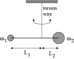
Fig. 2.1 Torsion balance used by Eötvös.

This is a sensitive device: any mismatch in forces or torques will have the setup either tilt or rotate a bit. Eötvös attached a tiny mirror to one of the arms of the rod. If you send a light beam on the mirror and let it reflect and be projected on a wall, then the smallest deviation in orientation (i.e. position) of the mirror will be amplified to create a large motion of the light spot on the wall.

In Eötvös experiment two forces are acting on each of the masses: gravity, proportional to \(m_g\), but also the centrifugal force \(F_c = m_i R \Omega^2\), the centrifugal force stemming from the fact that the experiment is done in a frame of reference rotating with the earth. This force is proportional to the inertial mass. The experiment is designed such that if the rod does not show any rotation around the vertical axis, then the gravitational mass and inertial mass must be equal. It can be done with great precision and Eotvos observed no measurable rotation of the rod. From this he could conclude that the ratio of the gravitational over inertial mass differed less from 1 than \( 5 \cdot 10^{-8}\). Currently, experimentalist have brought this down to \( 1 \cdot 10^{-15}\).

Note: the question is not if \(m_i / m_g\) is different from 1. If that was the case but the ratio would always be the same, then we would just rescale \(m_g\), that is redefine the value of the gravitational const \(G\) to make \(m_g\) equal to \(m_i\). No, the question is wether these two properties are separate things, like mass and charge. We can have two objects with the same inertial mass but give them very different charges. In analogy: if \(m_i\) and \(m_g\) are fundamentally different quantities then we could do the same but now with inertial and gravitational mass.

2.8. Examples & Exercises

Here are some examples and exercises that deal with forces. Make sure you practice IDEA.

Exercise 2.8

Who is strongest? Two strong boys try to keep a rope straight by each pulling hard at one end. A not so strong third person is pulling in the middle of the rope, but at an angle of 90\(^\circ\) to the rope. The two strong boys have the task to keep the deviation of the rope to a small value, set by you.

Or open the widget full screen

Interact with the widget about forces being vectors.

Exercise 2.9

You drop a stone from a height of 50m of the tower of the church. Calculate the velocity of the stone when it hits the ground (ignore friction). In the video (click on the image below) you will see on the left a quick and dirty solution, NOT using IDEA. The right hand side uses IDEA and Newton’s \(2^{nd}\) law.

Exercise 2.10

Or open the widget full screen

Inertia game. Mass has inertia; can you catch the red mass?

Exercise 2.11

Or open the widget full screen

Two point particles slide down a slope: one feels friction the other doesn’t. Can you analyse the situation and understand the graphs?

Exercise 2.12

Or open the widget full screen

What kind of forces are acting?

Exercise 2.13

Or open the widget full screen

A particle pulled by another.

Exercise 2.14

A point particle (mass \(m\)) is, from position \(z=0\), shot with a velocity \( v_0 \) straight upwards into the air. On this particle only gravity acts, i.e. friction with the air can be ignored. The acceleration of gravity, \(g\), may be taken as a constant.

The following questions should be answered.

1. What is the maximum height that the particle reaches?
2. How long does it take to reach that highest point?

Solve this exercise using IDEA.

1. Sketch the situation and draw the relevant quantities.
2. Reason that this exercise can be solved using F=ma (or dp/dt = F).
3. Formulate the equation of motion (N2) for m.
4. Classify what kind of mathematical equation this is and provide initial or boundary conditions that are needed to solve the equation.
5. Solve the equation of motion and answer the two questions.
6. Check your math and the result for dimensional correctness. Inspect the limit: $ F_{zw} \rightarrow 0 $.

First try it yourself (and try seriously) before peeking at the solution. Click solution to open a pdf.

Good Practice

It is a good habit to make your mathematical steps small: one-by-one. Don’t make big jumps or multiple steps in one step. If you make a mistake, it will be very hard to trace it back. Next: check constantly the dimensional correctness of your equations: that is easy to do and you will find the majorities of your mistakes.

Finally, use letters to denote quantities, including \( \pi \). The reason for this is:

1. letters have meaning and you can easily put dimensions to them;
2. letters are more compact;
3. your expressions usually become easier to read and characteristic features of the problem at hand can be recognized.

Exercise 2.15 (Acceleration of Gravity)

1. Find an object that you can safely drop from some height.
2. Drop the object from any (or several heights) and measure using a stop watch or you mobile the time from dropping to hitting the ground.
3. Measure the dropping height.

Find from these data the value of gravity's acceleration constant.

Don’t forget to first make an analysis of this experiment in terms of a physical model and make clear what your assumptions are.

Hint: think about the effect of air resistance and about the accuracy of measuring a time interval: is dropping from a small, a medium or a high height best? Any arguments?

Exercise 2.16 (Use numerical analysis to assess the influence of air friction)

If you want to learn also how to use numerical methods …

Try using an air drag force: \( F_{drag} = -A_\perp C_D \frac{1}{2} \rho_{air} v^2 \). With \( A_\perp \) the cross-sectional area of your object perpendicular to the velocity vector and \(C_D \approx 1 \) the drag coefficient (in real life it is actually a function of the velocity). \( \rho_{air} \) is the density of air which is about \(1.2 kg/m^3 \).

Write a computer program (e.g. in python) that calculates the motion of your object. See Solution with Python how you could do that.

Exercise 2.17 (Forces on your bike)

On a bicycle you will have to apply a force to the peddles to move forward, right? What force actually moves you forward, where is it located and who/what is providing that force?

1. Make sketch and draw the relevant force. Give the force that actually propels you a different color.
2. Think for a minute about the nature of this force: are you surprised?
   N.B. Consider while thinking about this problem: what would happen if you were biking on an extremely slippery floor?

To check your thoughts: click Riding a Bike .

Exercise 2.18 (Getting of the boat)

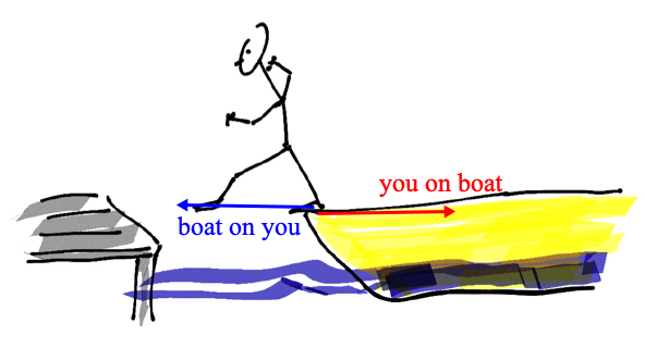
You are stepping from a boat onto the shore. Use Newton’s laws to describe why you will end up in the water.

N.B. A calculation is not required, but focus on the physics and describe in words why you didn’t make it to the jetty.

To check your thoughts: click Stepping off the boat .

Exercise 2.19 (Newton’s Laws)

Fig. 2.2 Stamp designs © Royal Mail Group Ltd^[1].

Close this book (or don’t peak at it ;-)) and write down Newton’s laws. Explain in words the meaning of each of the laws. Try to come up with several, different ways of describing what is in these equations.

Click Newtons Laws for a solution.

---

[1]

Cannot be reprinted without permission.