3. Analytical or Numerical

3.1. Calculus

Most of the undergraduate theory in physics is presented in the language of Calculus. We do a lot of differentiating and integrating. And for good reasons. The basic concepts and laws of physics can be cast in mathematical expressions, providing us the rigor and precision that is needed in our field. Moreover, once we have solved a certain problem using calculus, we obtain a very rich solution, usually in terms of functions. We can quickly recognize and classify the core features, that help us understanding the problem and its solution much deeper. As a simple example, let’s look at a particle of mass \(m\), that has initially (say at \(t=0\)) a velocity \(v_0\). For \(t>0\) the particle is subject to a force that is of the form \(F = - b v\). This is a kind of frictional force: the faster the particle goes, the larger the opposing force will be.

We would like to know what the position of the particle is as a function of time.

We can answer this question by applying Newton 2:

\[ m\frac{dv}{dt} = F \Rightarrow m\frac{dv}{dt} + bv = 0\]

Clearly, we have to solve a differential equation which states that if you take the derivative of \(v\) you should get something like \(- v\) back. From calculus we know, that exponential function have the feature that when we differentiate them, we get them back. So, we will try \(v(t) = A e^{-\mu t}\) with \(A\) and \(\mu\) to be determined constants.

We substitute our trial \(v\):

\[ m \cdot A \cdot -\mu e^{-\mu t} + b \cdot A e^{-\mu t} = 0\]

This should hold for all \(t\). Luckily, we can scratch out the term \(e^{-\mu t}\), leaving us with:

\[-m A \mu + Ab = 0\]

We see, that also our unknown constant \(A\) drops out. And, thus, we find

\[ \mu = \frac{b}{m} \]

Next we need to find \(A\): for that we need an initial condition, which we have: at \(t=0\) is \(v=v_0\). So, we know:

\[v(t) = A e^{-\frac{b}{m}t} \text{ and } v(0)=v_0\]

From the above we see: \(A = v_0\) and our final solution is:

\[v(t) = v_0 e^{-\frac{b}{m}t}\]

From the solution for \(v\), we easily find the position of \(m\) as a function of time. Let’s assume that the particle was in the origin at \(t=0\), thus \(x(0)=0\). So, we find for the position

\[\frac{dx}{dt} \equiv v = v_0 e^{-\frac{b}{m}t} \Rightarrow x = v_0 \cdot \left ( -\frac{m}{b}e^{-\frac{b}{m}t} \right ) + B\]

We find \(B\) with the initial condition and get as final solution:

\[x(t) = \frac{m v_0}{b} \left ( 1 - e^{-\frac{b}{m}t} \right ) \]

If we inspect and assess our solution, we see: the particle slows down (as is to be expected with a frictional force acting on it) and eventually comes to a stand still. At that moment, the force has also decreased to zero, so the particle will stay put.

3.2. Numerical

Of course, now that we have the analytical solution, there is nothing to add or gain from a numerical analysis. Nevertheless, it is instructive to see how we could have dealt with this problem using numerical techniques. One way of solving the problem is, to write a computer code (e.g. in python) that computes from time instant to time instant the force on the particle, and from that updates the velocity and subsequently the position.

Here is the approach. First, we rewrite the differential equation for \(v\) into a finite difference equation. That is, we go back to how we came to the differential equation:

\[ m \lim_{\Delta t \rightarrow 0} \frac{v(t+\Delta t) - v(t)}{\Delta t} = F \]

On a computer, we can not literally take the limit of \(\Delta t\) to zero, but we can make \(\Delta t\) very small. If we do that, we can rewrite the difference equation (thus not taken the limit):

\[ v(t+ \Delta t) = v(t) + \frac{F}{m}\Delta t \]

This expression forms the heart of our numerical approach. We will compute \(v\) at discrete moments in time: \(t_i = 0, \Delta t, 2\Delta t, 3\Delta t, ...\). We will call these values \(v_i\). Note that the force can be calculated at time \(t_i\) once we have \(v_i\). Thus our calculation scheme becomes (with \(F = -b v\)):

\[v_{i+1} = v_{i} - \frac{b}{m}v_i \Delta t\]

Similarly, we can keep track of the position:

\[\frac{dx}{dt} = v \Rightarrow x_{i+1} = x_i + v_i \Delta t\]

With the above rules, we can write an iterative code, which reads something like:

for i is 1 to N:
    compute new v: v[i+1] = v[i] - b/m*v[i]*dt
    compute new x: x[i+1] = x[i] + v[i]*dt

Here is a python code that gives the starting values for \(x\) and \(v\) for given values of \(b, m\) and \(dt\).

import numpy as np
import matplotlib.pyplot as plt

# Parameters
m = 1.0           # mass
x0 = 0.0          # initial position
v0 = 1.0          # initial velocity
dt = 0.01         # time step
T = 10.0          # total time
b = 0.3           # friction coefficient

# Define force function: friction force F = -b v
def force(x, v, t):
    return -b * v

# Time array
steps = int(T/dt)
t = np.linspace(0, T, steps+1)

# Arrays to store position and velocity
x = np.zeros(steps+1)
v = np.zeros(steps+1)

# Initial conditions
x[0] = x0
v[0] = v0

# Euler forward integration
for n in range(steps):
    a = force(x[n], v[n], t[n]) / m
    v[n+1] = v[n] + a * dt
    x[n+1] = x[n] + v[n] * dt

# Plot results
plt.figure(figsize=(10,4))
plt.subplot(1,2,1)
plt.plot(t, x)
plt.xlabel('Time')
plt.ylabel('Position')
plt.title('Position vs Time')

plt.subplot(1,2,2)
plt.plot(t, v)
plt.xlabel('Time')
plt.ylabel('Velocity')
plt.title('Velocity vs Time')

plt.tight_layout()
plt.show()

In the graph, we have plotted both the analytical solution and the numerical one. As can be seen, if we make \(dt\) sufficiently small, the numerical solution can not be distinguished from the analytical one.

3.3. More difficult example

In the above, the friction force was proportional to the velocity. What if we make the force more realistic? For instance, let’s consider a small hail stone that comes falling out of the sky. We will assume that the hail stone is formed in a cloud at a height of 1km above the ground. Furthermore, we will take that the stone drops from that height with zero initial velocity. Finally, we will assume that the problem is 1-dimensional: the hail stone drops vertically down and experiences only gravity, buoyancy and air-friction. The situation is sketched in Fig. 3.1.

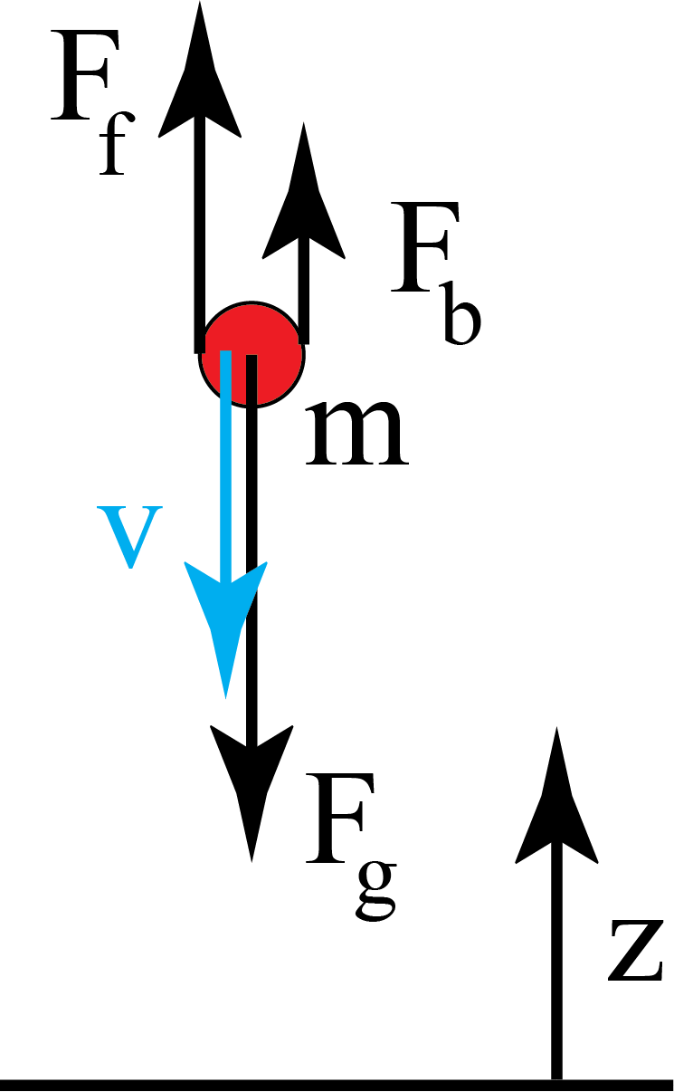
Fig. 3.1 .

There are three forces acting on the hail stone: gravity, \(F_g = - mg = \rho_p V_p g\), buoyancy, \(F_b = \rho_{air} V_p g\) and air friction. The latter can not be written down from a first-principles argument. We have to use here an empirical relation. We will use (taken the hail stone as a spherical particle with diameter \(D\)):

(3.1)\[F_f = -C_D \frac{\pi}{4}D^2 \frac{1}{2}\rho_{air} |v| v\]

with \(C_D\) the so-called drag coefficient that can be approximated by e.g.

(3.2)\[C_D = \frac{24}{Re} \left ( 1 + 0.15 Re^{0.678} \right)\]

and

(3.3)\[Re = \frac{\rho_{air} v D}{\mu_{air}}\]

\(\rho_{air} = 1.2 kg/m^3\) is the density of air and \(\mu_{air} = 1.8 \cdot 10^{-5} kg/(m\cdot s) \) the viscosity of air.

So, we have to deal with a much more complicated expression for the friction force, making integration of N2 virtually impossible. However, a numerical approach does not change by much. Now we have to evaluate a more complex friction force, but the entire approach remains the same.

Note, that for \(Re<1\) the friction force tends to \(F_f \propto -v\) as we had in the previous example. Therefor, we will compare our numerical solution with the analytic one that assumes that the friction force is proportional to \(v\).

3.3.1. Simulation of a falling hail stone: friction versus no friction with the surrounding air

Show code cell source

Hide code cell source

import plotly.graph_objects as go
import numpy as np

################ Code used for physics ################
# Define constants
rho_p   = 915
rho_air = 1.2
mu_air  = 1.8e-5
D       = 2.5e-3
H       = 1e3
g       = 9.813
v0      = 0
z0      = H

m   = np.pi/6 * D**3 * rho_p
A   = np.pi/4 * D**2
Vol = np.pi/6 * D**3

dt  = 1e-2
Ndata = 501

# Update D values
def recalc(D):
    '''Function to recompute all values that depend on D'''
    D   = D
    m   = np.pi/6 * D**3 * rho_p
    A   = np.pi/4 * D**2
    Vol = np.pi/6 * D**3
    return D, m, A, Vol

def CD(v,D):
    '''Function to compute the drag coefficient'''
    Re = rho_air * np.abs(v) * D / mu_air
    if Re < 1e-6:
        Re = 1e-6
    CD = 24./Re*(1 + 0.15 * Re**0.678 )
    return CD

def force(v,D,m,Vol,A):
    '''Function to compute the force'''
    f = -m*g + rho_air*Vol*g - CD(v,D)*A*1/2*rho_air*np.abs(v)*v
    return f

def velo(D):
    '''Parametrized function to determine t, v and v without friction used in plotting'''
    recalc(D)
    v = []
    v_nofriction = []
    z = []
    t = []
    v.append(v0)
    v_nofriction.append(v0)
    z.append(z0)
    t.append(0)
    teller = 0
    while teller < Ndata:
        teller = teller + 1
        t.append(teller*dt)
        v_new = v[teller-1] + force(v[teller-1],D,m,Vol,A)/m*dt
        z_new = z[teller-1] + v_new * dt
        v.append(v_new)
        z.append(z_new)
        v_nofriction.append(-g*teller*dt)
    return t, v, v_nofriction

# Compute initial values                             
[t,v,v_nofriction] = velo(D)

################ Code used for Interactive Plot ################
line_red = '#e96868' # red line
line_blue = '#68a0e9' # blue line
fig = go.Figure()

# Define the steps for the slider and an empty array of the minimum values used later for setting the y-axis range
slider_steps = np.arange(0.1,5,0.1)
vmin = np.zeros_like(slider_steps)

for ind,val in enumerate(slider_steps):
    # Rescale D to meters and compute values
    D = val * 1e-3
    recalc(D)
    [t,v,v_nofriction] = velo(D)
    vmin[ind] = min(v)

    # Add the trace with friction
    fig.add_trace(
        go.Scatter(
            visible=False,
            x = t,
            y = v,
            line = dict(color=line_red),
            mode = 'lines',
            name = 'friction'))
    
    # Add the trace without friction
    fig.add_trace(
        go.Scatter(
            visible=False,
            x = t,
            y = v_nofriction,
            line = dict(color=line_blue),
            mode = 'lines',
            name = 'no friction'))
    
    # Update the y-axis range
    fig.update_yaxes(range=[2 * v[-1], 0], title_text=r'v(t)')

base_traces = 0 
traces_per_step = 2 # Number of traces per value of a

# Show the traces for one value of a when loading the plot (initial setup)
active_index = slider_steps.shape[0]//2

# Set the traces for the active value of D to visible
for i in range(traces_per_step):
    current_index = int(base_traces + active_index*traces_per_step + i)
    fig.data[current_index].visible = True

steps = []
for i in range(0, slider_steps.shape[0]):

    # Make only the traces for the current value of a visible
    visarray = [False] * len(fig.data)
    visarray[0:base_traces] = [True] * base_traces

    current_index = int(base_traces + i * traces_per_step)
    next_idx = int(base_traces + (i+1) * traces_per_step)
    visarray[current_index:next_idx] = [True] * traces_per_step

    # Define content of the slider step
    step = dict(
        method="update",
        args=[
            {"visible": visarray},
            {"yaxis.range": [2 * vmin[i], 0]},
            {"yaxis.titletext": r'v(t)'}
        ],
        label=str(round(slider_steps[i], 1))
    )
    
    steps.append(step)

sliders = [dict(
    active = active_index,
    currentvalue = {"prefix": "diameter: ", "suffix": " mm", "font": {"size": 20}},
    steps = steps
)]

fig.update_layout(
    sliders=sliders,
    legend_title="Legend"
)

fig.update_xaxes(title_text=r't [s]', range=[0, 5])

# Update yaxis properties
fig

3.4. Exercises

Exercise 3.1

A point particle of mass m, feels a force \(F(x) = - F_0 \;\text{ sign}(x) \; e^{-|x|/L}\). Here, \(\text{sign}(x)\) denotes the ‘sign-function’. It is +1 for \(x>0\), -1 for \(x<0\) and 0 for \(x=0\).

The particle is at \(t=0\) at \(x=0\) and has a velocity \(v(0) = v_0\).

Write a simulation that determines the position of the particle as a function of time: \(x(t)\). The problem is 1-dimensional. Take \(m=1 kg, L=1m, F_0 = 2N\) and vary \(v_0\) between 1.5 and 2.5m/s. Set the value of \(dt\) in your code to 0.001 (s) and simulate about 60 seconds.

Inspect what happens for initial values of the velocity around 2 m/s. Any clue what this means? If not: don’t worry. You will get the ‘tools’ when we discuss work and energy.

Exercise 3.2

In the examples so far, we looked at 1-dimensional problems, for instance, the falling hail stone. Given the expression for the drag force with the algebraic formula for the drag coefficient, an analytical approach could be tried, although a numerical one turned out to be straightforward. This changes, when we deal with a 2-dimensional trajectory.

The standard classical mechanical example is that of the ‘canon ball’: a point mass of mass m is shot into the air from \(z=0\) with initial velocity \(v_0\) at an angle \(\alpha\) with the horizontal. The only force taken into account is gravity and the question is: “at what value does the ball travel furthest?” This is a 2-dimensional, which makes it in principle more complicated. However, in this case, the equations for the motion in the horizontal and vertical direction are uncoupled and can be solved separately. it is relatively simple to show that the path is longest at \(\alpha = 45^\circ\), independent of the initial velocity of the ball.

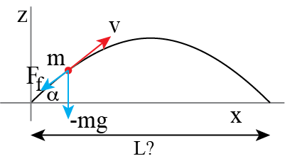
But what if we do take air friction into account? The equation of motion is:

\[m\frac{d\vec{v}}{dt} = -m\vec{g} - C_D \frac{\pi}{4}D^2 \frac{1}{2} \rho_{air} v \vec{v} \]

and we use for the drag coefficient, just like before:

(3.4)\[C_D = \frac{24}{Re} \left ( 1 + 0.15 Re^{0.678} \right)\]

and

(3.5)\[Re = \frac{\rho_{air} v D}{\mu_{air}}\]

\(\rho_{air} = 1.2 kg/m^3\) is the density of air and \(\mu_{air} = 1.8 \cdot 10^{-5} kg/(m\cdot s) \) the viscosity of air.

But now, the problem is two dimensional and the two directions are coupled! This is a consequence of the quadratic nature of the friction force: it contains the value of the velocity, that is both components:

\[\begin{split} \begin{split} F_{f,x} &= -C_D(v) \frac{\pi}{4}D^2 \frac{1}{2} \rho_{air} v . v_x \\ F_{f,y} &= -C_D(v) \frac{\pi}{4}D^2 \frac{1}{2} \rho_{air} v . v_y \end{split} \end{split}\]

This makes analytical solution rather difficult. However, with a numerical approach, the same ideas as for a 1-d case can be used and extension is straight forward.

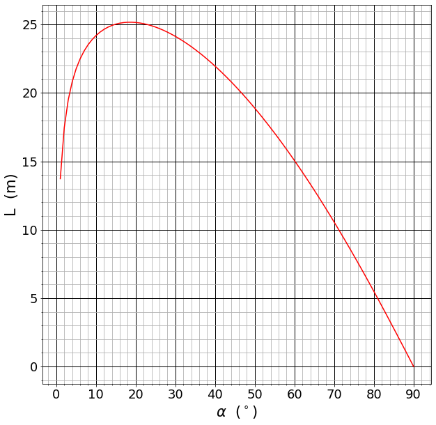
Write a computer code for the case of a spherical sand particle of 1 mm (density 2.5 10\(^3\) kg/m\(^3\)) that is shot at 10m/s at an angle \(0 \lt \alpha \lt 90^\circ\) with the horizontal and find the maximum distance it can travel (and the angle at which that happens).

You should find something like shown in the graph below.

Exercise 3.3

A pendulum is by most people known for its ‘clock work’. In old fashioned clocks it swings back and force at a constant period. The small friction it encounters is balanced by a driving force, usually coming from weights that slowly move downwards due to gravity.

However, a pendulum can show complex motion if the driving force is not a constant. A very simple example is a pendulum, that experiences some friction that is linearly related to the velocity of the bob and a driving force that is a cosine of time. Mathematically, this can be described by the following equation of motion:

\[m \ddot{x} = -\gamma \dot{x} - \alpha \sin (x) + A \cos (2\pi ft) \]

If we analyse this equation, we see on the left hand side ‘ma’ and on the right hand side the forces. That is: friction, the effect of gravity and the driving force. In the current exercise, we set:

\[ \gamma = 0.1 s^{-1}, \alpha = 1 rad/s^2, A = 1 rad/s^2 \text{ and } 2\pi f = 1 s^{-1} \]

This symplifies the equation of motion to

\[\ddot{x} = -0.1 \dot{x} - \sin (x) + \cos (t) \]

The initial conditions are: \(x(0) = 0\) and \(\dot{x}(0) = 2.0 \)

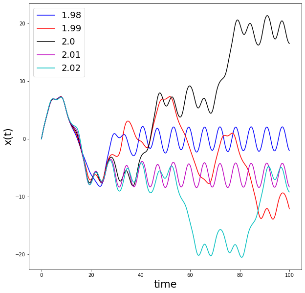
Write a numerical code that solves the above problem and plot \(x(t)\) for different values of \(\dot{x}(0)\), namely 1,8, 1.9, 2.0, 2.1, 2.2.

You will experience, that small changes in the initial condition have large consequences for the trajectory \(x(t)\), which is a characteristic of chaotic systems. And indeed, this pendulum shows chaotic behavior. It is virtually impossible to solve the equation of motion analytical, but a numerical solution is made relatively easily.

Note that for a reliable solution, better numerical schemes than the one we are using here are needed. An example of five different initial conditions giving five different solutions, but now made with higher order schemes, is given in the figure below.