Cracks in Classical Mechanics

15. Cracks in Classical Mechanics#

As the years progressed, Classical Mechanics developed further and further. So, in the first half of the nineteenth century it felt like classical mechanics was an all encompassing theory and that physics would become a discipline of working out problems based on a well-established, complete theory. But that wasn’t going to be the case at all. Around 1850-1860 several cracks in the theory started to become visible. And they were fundamental!

Already in the 18$^{th}$ century, work was done on what we call the kinetic theory of gases. The Swiss scientist Daniel Bernoulli proposed that gases were a large collection of molecules, i.e tiny particles moving in all directions. According to Bernoulli, their collision with walls was felt macroscopically as pressure and their averaged kinetic energy was in essence the temperature of the gas.

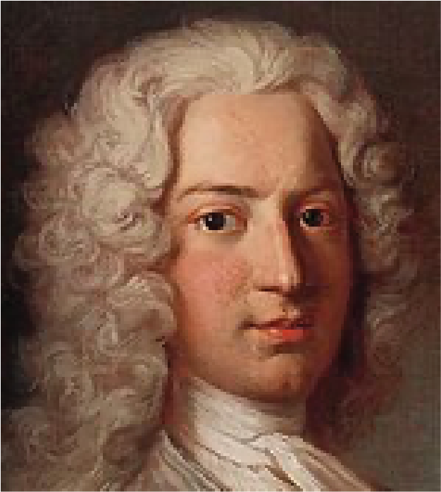
../_images/DanielBernoulli.png — Fig. 15.1 Daniel Bernoulli (1700-1782).
From Wikimedia Commons (https://commons.wikimedia.org/
wiki/File:Portr%C3%A4t_des_Daniel_Bernoulli_
(cropped).jpg), licensed under CC-BY-SA 4.0.#

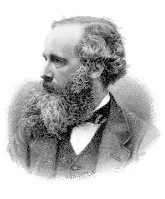
../_images/JamesClerkMaxwell.png — Fig. 15.2 James Clerk Maxwell (1831-1879).
From Wikimedia Commons, public domain.#

It took a while before these ideas were accepted, partly because the law on conservation of energy was not fully developed. Moreover, people had difficulty accepting that a molecular level collisions could be perfectly elastic.

With the further development of Thermodynamics, the kinetic theory of gases also was refined. In 1856, August Krönig came up with a simple kinetic model for gases in which he only considered the possibility of translational motion of the molecules. In essence, he treated gas molecules as point particles. A year later, in 1857, Rudolf Clausius incorporated the possibility of rotation and vibrations. Two years after this, James Clerk Maxwell continued along this line. He found the velocity distribution of the molecules and established a firm connection between temperature and the average kinetic energy of a molecule.

Specific heat of gases
However, he also noted that the theoretical predictions were not in line with experiments. What was the problem? For ideal gases, we have the ideal gas law: $pV = nRT$ with $n$ the number of moles of the gas in question. Or written in terms of number of molecules, $N$ it reads as: $pV = NkT$, $k$ being the Boltzmann constant.

The ideal gas law helps in understanding that if we compress a given amount of gas, we may expect that the pressure goes up. But we also see that this depends on whether or not the temperature changes. And in principle it will.

If we would do a compression experiment with a fixed number of molecules, $N$, and we would compress the gas such that no heat can escape from the container, then the changes in temperature, volume and pressure are such that $p V^\gamma = const$. This is called adiabatic compression. The quantity $gamma$ is the ratio of the specific heat at constant pressure over the specific heat at constant volume. Both these quantities are easily measured in experiments and, hence, $\gamma$ can be found for many gases.

The kinetic theory predicts $\gamma$ for various classes of gases. For instance, for monatomic gasses as Helium is $5/3 \approx 1.667$; for diatomic gases, such as Oxygen or Hydrogen, it should be $9/7 \approx 1.286$. And so on. Moreover, $\gamma$ does, according to the kinetic theory, not depend on temperature.

Gas	T (K)	c_p/c_v	kin.gas.th.
He	293	1.663	1.667
Ne	293	1.667	1.667
Kr	293	1.656	1.667
Ne	293	1.667	1.667
Br₂	293	1.28	1.286
Cl₂	293	1.34	1.286
H₂	293	1.405	1.286
N₂	293	1.40	1.286
O₂	293	1.395	1.286

As we see, for the noble gases it is quite ok (at $T=293K$!), but not so for the diatomic gases.

For really high temperatures (~2000K) for both $O_2$ and $H_2$ $\gamma$ is close to 1.286. But if we go to low temperature, their respective $\gamma$’s increase and $H_2$ reaches a value of 1.66!

Maxwell concluded, that the laws of classical mechanics could not be the final answer.

As we have seen when discussing Rutherford’s experiment, in the early twentieth century more cracks became visible. These led scientists to Quantum Mechanics.

15.1. The problem with Maxwell’s equations#

In the early 1860s Maxwell extended Ampères law, in combination with Gauss and Faraday laws. This led to four coupled differential equations describing the generation of electro-magnetic fields from charges and currents. They are now just known as the Maxwell equations. They read in modern (differential) notation as follows for the electric $\vec{E}(\vec{x},t)$ and magnetic $\vec{B}(\vec{x},t)$ field in free space

\[\begin{split} \begin{array}{rcl} \nabla \cdot \vec{E} &=& \frac{\rho}{\epsilon_0}\\ \nabla \cdot \vec{B} &=& 0\\ \nabla \times \vec{E} &=& -\frac{\partial \vec{B}}{\partial t}\\ \nabla \times \vec{B} &=& \mu_0\vec{J}+ \epsilon_0 \mu_0 \frac{\partial \vec{E}}{\partial t} \end{array} \end{split}\]

With $\rho(\vec{x})$ the charge density distribution and $\vec{J}(\vec{x},t)$ the electric current density, and constants $\epsilon_0$ the vacuum permittivity and $\mu_0$ the vacuum magnetic permeability. Or in integral notation

\[\begin{split} \begin{array}{rcl} \oint \vec{E}\cdot d\vec{A} &=& \frac{q}{\epsilon_0}\\ \oint \vec{B}\cdot d\vec{A} &=& 0\\ \oint \vec{E}\cdot d\vec{\ell} &=& -\frac{d \Phi_B}{d t}\\ \oint \vec{B}\cdot d\vec{\ell} &=& \mu_0 I+ \epsilon_0 \mu_0 \frac{d \Phi_E}{d t} \end{array} \end{split}\]

You will learn all about Maxwell’s equations in classes like Electromagnetism and Advanced Electrodynamics. The mathematics of these equations is quite difficult as each equation is $3D+t$ and the equations are coupled.

In vacuum

In vacuum ($\rho=0$ and $\vec{J}=0$) we can take the curl of the third equation, use the curl identity $\nabla \times (\nabla \times \vec{E})= \nabla (\nabla \cdot \vec{E})-\nabla^2 \vec{E}$, the first, and the fourth equation to arrive at the wave equation

\[ \nabla^2 \vec{E} - \epsilon_0 \mu_0 \frac{\partial^2 \vec{E}}{\partial t^2}=0 \]

This equation describes the propagation of the electric field through vacuum (you can of course derive the same equation for the magnetic field). In the wave equation a second derivative in space is coupled with a second derivative in time. The solution to this differential equation is $\vec{E}(\vec{x},t)\propto \cos(\vec{k}\cdot \vec{x}-\omega t)$, with the wave vector $\vec{k}$ pointing the direction of propagation and with magnitude $k=2\pi/\lambda, \omega = 2\pi \nu$ and $\nu \lambda =c$ with the frequency of oscillation $\nu$ and wavelength $\lambda$. You will learn more about this in courses likeElectromagnetism and Introduction to Waves. Light is identified as an electro-magnetic wave and from this equation the wave velocity is clearly

\[ \frac{1}{\sqrt{\epsilon_0 \mu_0}}\equiv c=2.998\cdot 10^8\ m/s \approx 300,000\ km/s \]

If the Maxwell equations are laws of physics all inertial observers must be able to write down the equation in the same form. Therefore for an observer $S'$, traveling at constant velocity $V\hat{x}$ with respect to $S$, we would write down the wave equation for a field that propagates only along the $x$-direction with amplitude in the $z$-direction (without loss of generality) $\vec{E}=(0,0,E_z(x,t))$ as

\[ \frac{\partial^2 E'_{z'}}{\partial x^{'2}} - \epsilon_0 \mu_0 \frac{\partial^2 E'_{z'}}{\partial t^{'2}}=0\ (*) \]

This has exactly the same form as for $S$ which is good if it should represent a physical law. However, for $S'$ the speed of the wave is also given by $c=\frac{1}{\sqrt{\epsilon_0 \mu_0}}$. As the speed is covered by universal constants $\epsilon_0, \mu_0$, the speed is the same of $S$ and $S'$ or in other words $c=c'$!
This is not what should happen! From the Galileo Transformation we know that we should find the same form, but with $c'=c-V$ the relative velocity of the two observers.

The Navier-Stokes equations are Galileo invariant as shown earlier, but the Maxwell’s equation are not!

So, let’s the more formal route as we have done with Navier-Stokes and see what happens.
For a transformation $S\to S':\ x'=x-Vt,t'=t$ we need to transfer the partial derivatives to the new coordinates, repeating what we found earlier, by applying the chain rule $$\frac{\partial f(x(x',t'))}{\partial x} = \frac{\partial f}{\partial x'}\frac{\partial x'}{\partial x} + \frac{\partial f}{\partial t'}\frac{\partial t'}{\partial x}$$

and using $\frac{\partial x'}{\partial x}=1$, $\frac{\partial t'}{\partial x}=0$, $\frac{\partial t'}{\partial t}=1$ and $\frac{\partial x'}{\partial t}=-V$, we find

\[\begin{split} \begin{array}{rcl} \frac{\partial}{\partial x} &=&\frac{\partial}{\partial x'}\\ \frac{\partial}{\partial t}&=& \frac{\partial}{\partial t'}-V \frac{\partial}{\partial x'} \end{array} \end{split}\]

Application of the same trick for the second derivative gives us

\[\begin{split} \begin{array}{rcl} \frac{\partial^2}{\partial x^2} &=& \frac{\partial^2}{\partial x^{'2}} \\ \frac{\partial^2}{\partial t^2} &=& \frac{\partial^2}{\partial t^{'2}}- 2V \frac{\partial^2}{\partial x'\partial t'} + V^2 \frac{\partial^2}{\partial x^{'2}} \end{array} \end{split}\]

If we apply the coordinate transformation from $S\to S'$ the wave equation reads thus as

\[ \frac{\partial^2 E_z}{\partial x^{'2}}-\frac{1}{c^2}\frac{\partial^2 E_z}{\partial t^{'2}}-\frac{V^2}{c^2}\frac{\partial^2 E_z}{\partial x^{'2}}+ \frac{2V}{c^2}\frac{\partial^2 E_z}{\partial x' \partial t'}=0 \]

Now, we still need to find a transformation $E_z\to E'_{z'}$ (and $c'\to c)$ trying to retrieve the general form of the wave equation, but there is no such transformation. Therefore the wave equation of electromagnetic waves is not Galilei invariant at all!

The solution is that the Galilei transformation does not govern the physical laws, but the Lorentz transformation as we will see in the rest of the course. However, the difference between these two transformation is only relevant for very high speeds. Equation $(*)$ is indeed Lorentz invariant.

NB: The Navier-Stokes equation is not Lorentz invariant, and therefore needs a correction for high velocities. If any equation is not Lorentz invariant, this means it does not tell us the full picture of physics, something must be missing! For example Schrödinger directly knew that his equation was not the end, as it is not Lorentz invariant - only the extension by Paul Dirac made it so.

15.1.1. Hypothesis of the aether#

As light is a wave, people naturally thought there must be a medium to transport the wave, something must be oscillating. Vacuum was considered nothing, not something. A water wave, needs water as medium to transport the wave; the water oscillates. Or take sound waves, they need gas, liquid or a solid to oscillate. What could be the medium that light, electromagnetic waves, use to oscillate? This medium must be all around us, in the space between the sun and earth, just everywhere. To save the Galilei invariance of Maxwell’s equations this also needs to be a very special kind of medium that behaves differently than other media. This strange hypothetical medium was termed aether. The search for the properties of the aether lead to the Michelson-Morley experiment - which showed that there was no aether at all! Lorentz and Fitzgerald found an ad hoc way to save the day by postulating an adapted version of the Galilei transformation and a contraction of length respectively. Later more about that, and how Einstein showed that all of this ad hoc business is not needed, things follow directly from his second axiom.

15.2. The Michelson-Morley experiment#

The Michelson-Morley experiment was performed in between 1880-1890 to investigate properties of the hypothetical aether. The experiment returned a null-result, i.e. there was no sign of the existence of the aether - and to this day there is none.

The idea is to check the speed of light for two observers $S$ and $S'$. One is moving with respect to the other with the highest possible speed, the orbit speed of the earth around the sun $\sim 30$ km/s. Of course, that is still only $10^{-4}$ compared to 300,000 km/s of the speed of light but the effects could be measured spectroscopically by interference.

The experiment essentially consists of a Michelson interferometer. Light is send to a 50/50 beam splitter such that half of the light is reflected towards arm $L_1$ and half is transmitted to arm $L_2$. The mirrors at the end of each arm reflect the light back. On the way back again half of the light is transmitted and reflected at the beamsplitter, such that half of the light from both arms is now traveling downwards towards the image plane/camera. At the image plane the light from both arms form an interference pattern, depending on the path length difference induced by the difference of $L_1-L_2$.

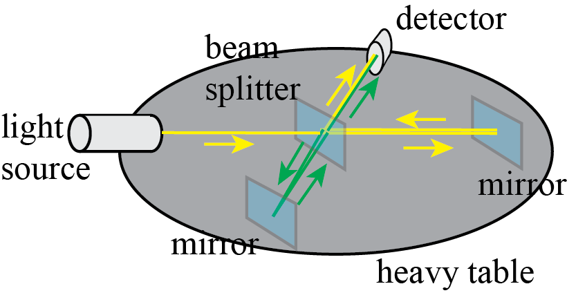
../_images/MichelsonMorleyExp.png — Fig. 15.3

Michelson & Morley setup#

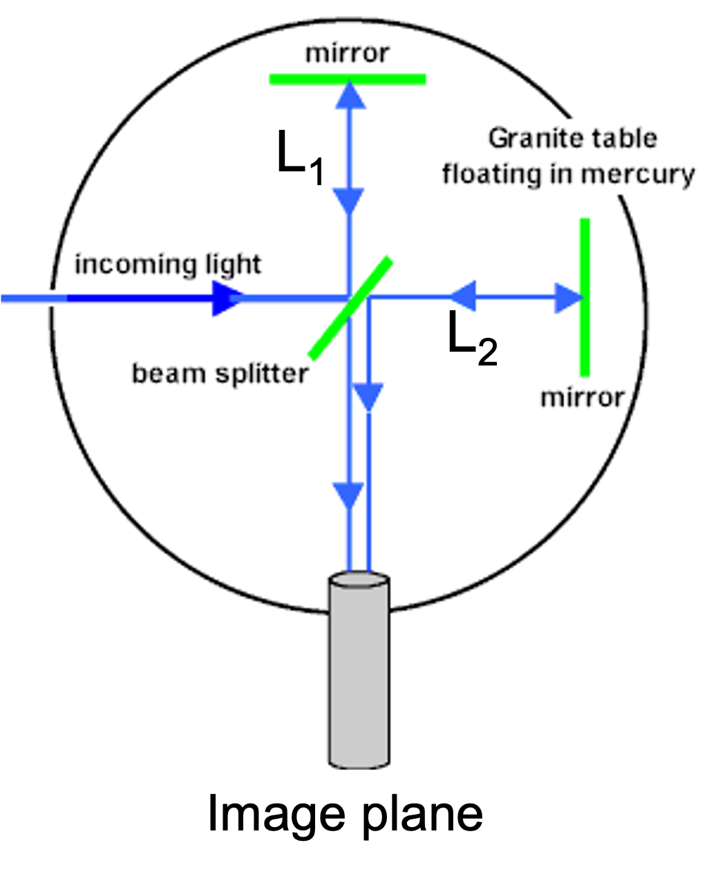
../_images/MM-setup.png — Fig. 15.4 From Space and Motion,
licensed under CC-BY-SA-NC 3.0.#

The whole setup is mounted for stability on a heavy table that is floating in liquid mercury, to reduce vibrations coupling to the setup. If now one arm is parallel to the earth’s orbit with $V=30$km/s, while the other is perpendicular to it, there will be some phase shift between the two arms $\Delta \lambda_1$. If we rotate the setup by 90 degree (easily done in the mercury bath, although not really healthy), then the roles of $L_1$ and $L_2$ are exchanged, leading to another phase shift $\Delta \lambda_2$. Therefore, after rotation the fringe pattern on the image plane/camera should shift as

\[ \Delta \phi=2\pi\frac{\Delta \lambda_1 - \Delta \lambda_2}{\lambda} = 2\pi\frac{(L_1+L_2)}{\lambda}\frac{V^2}{c^2} \]

If we fill in the numbers $\lambda =550$ nm, $L_1+L_2=11$ m and $V^2/c^2=10^{-8}$ this results in an expected $\Delta \phi=0.4 \pi$. However, Michelson and Morely found only $\Delta \phi \leq 0.01\pi$. The experiment to find the aether failed.

Physics was is serious trouble until 1905.

NB: Back in the days, white light was used for the actual measurement and monochromatic coherent light of e.g. a sodium lamp for alignment. As white light produces a colored interference pattern which is much easier to observe visually. Otherwise temperature changes or vibrations, resulted in constant fringe drift. Today monochromatic laser light can be used in combination with environmental temperature control better than to 0.1 C and sensitive CCD cameras. Today experiments have confirmed the null-result of Michelson and Morley but to much better precision. The anisotropy in the speed of light is $c_\perp / c_{||}\leq 10^{-17}$.

Although the proposed hypothetical medium aether (or ether) does not exist, as proven a long time ago, the terminology did not drop from everyday language.

15.3. Einstein’s axioms#

In 1905 Einstein formulated his special theory of relativity with the article Zur Elektrodynamik bewegter Körper, Annalen der Physik, 17:891-921, 1905. He choose the Maxwell equations and the Michelson Morely experiment as a starting point for this argument to arrive at

The laws of physics are the same in all inertial frames of reference.
The velocity of light in vacuum is the same in all inertial frames.

That does not sound like a lot or world changing, but it certainly was. You can directly see that the second axioms violates Galilean addition of velocities, but that is what was found experimentally!

If you think these two axioms stubbornly thorough and take their consequences seriously, things get hairy. We will do this.

Extra reading with a historic perceptive. In a 200 page book Wolfgang Pauli -Theory of Relativity, Dover (The original German version is available online Relativitätstheorie - summaries all that was known about special relativity as a request made by his PhD advisor Arnold Sommerfeld. It is worth a read, although the notation is a bit outdated.

Extra reading Hoe de ether verdween uit de natuurkunde. This article by Jos Engelen in the Nederandse Tijdschrijft voor Natuurkunde explains the Michelsen-Morley experiment, places it into historic perspective and then adds the work of Lorentz, Poincaré and Einstein leading to the Lorentz transformation.

15.4. Exercises#

Exercise 15.1

Assume the Michelson-Morley experiment uses arms of length $L$ = 11 m and an aether wind speed $v$ due to the motion of the earth around the sun.
Distance earth-sun: $150 \cdot 10^6$km.
Calculate the expected time difference $\Delta t$ between light traveling parallel and perpendicular to the aether wind.

The sun itself is orbiting the center of our Milky Way at an even higher speed: 250 km/s. What would this mean for the expected time difference in the Michelson and Morley experiment?

Note: in the experiment of 1887, Michelson and Morley had used multiple mirrors in their set up for each of the two light beam paths to make the traveling length of the light, from the splitter to the mirror and the edge of the table and back, much longer than only the radius of the table and back. This is how they achieved a path length of 11m. The table itself was of course not of a diameter of 22m.

15.5. Answers#

Solution to Exercise 15.1

The orbit of the earth around the sun is almost circular. Thus, we can estimate the velocity of the earth as $v = \frac{2\pi R}{T}$ with $R=150 \cdot 10^6$ km and $T$ = 1 year = 31.6 $10^6$ s. This gives $V$ = 30 km/s.

We compute the traveling time from light leaving the beam splitter, reflecting at the mirror on the side of the table and reaching the beam splitter again. The rest of the path is identical for both light beams and does not lead to a time difference.

time for light parallel to $V$: one part - tail wind from eather and velocity (according to Classical Mechanics with Galilei Transformation) $c+V$. Other part: head wind with velocity $c-V$. Thus travelling time:

\[t_{//} = \frac{L}{c-V} + \frac{L}{c+V} = \frac{2L}{c} \frac{1}{1-\frac{V^2}{c^2}}\]

time to travel perpendicular to $V$:

\[t_\perp = \frac{L}{\sqrt{c^2 - V^2}} + \frac{L}{\sqrt{c^2 - V^2}} = \frac{2L}{c} \frac{1}{\sqrt{1-\frac{V^2}{c^2}}}\]

Putting in the numbers, we find $ \Delta t = 3.67 \cdot 10^{-16}s$

This time difference may be way to small to measure. And indeed, no ‘stop-watch’ experiment will work. But Michelson & Morley used interferometry, i.e. interference of light. So, relevant is the difference in phase of the two light beams. This can be assessed by turning the time difference into a length: $\Delta s = c \Delta t =1.1 \cdot 10^{-7}$m. Compare this to the wave length of the (yellow) light used by Michelson and Morley: $\lambda \approx 500 nm = 5 \cdot 10^{-7} m$. Conclusion: the expected time difference is well in reach of interferometry.

If we take the velocity of the sun around the center of the Milky Way, we get $ \Delta t = 2.55 \cdot 10^{-14}s$ and the corresponding length difference $\Delta s = c \Delta t = 7.6 \cdot 10^{-6}$m.