9. Oscillations

9.1. Periodic Motion

There are many, many examples of periodic systems. We see them in physics, like the orbit of planets around their star. We find them in biology, in chemistry, in economics. They show up in daily life: the day-night rhythm, the tides, children on a swing, your heart-beat. Periodic motions are by definition motions that repeat themselves after a fix period of time, usually called ‘the period’.

A specific class of periodic motion is formed by the oscillations. All oscillations are period, but not all periodic motion is an oscillation. An oscillation is moving back and forth around an equilibrium position. They are often caused by the presence of restoring forces: forces that try to push the system towards the equilibrium position. A form of inertia causes the system to overshoot. The restoring force reverses in direction to push the system back after the overshoot.

A few simple examples will illustrate the above. The merry go round is a periodic motion, but not an oscillation.

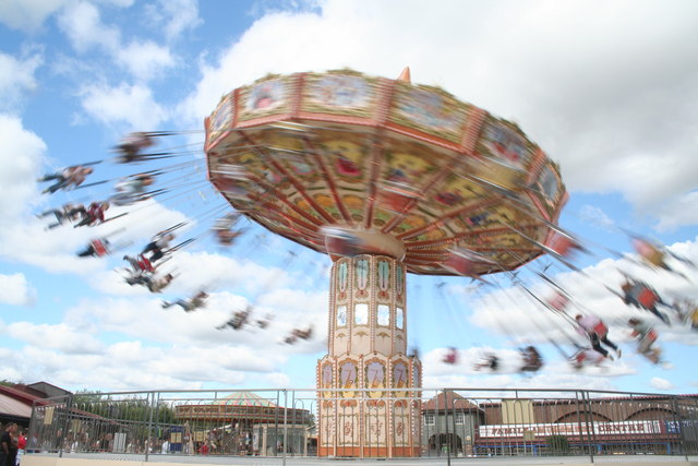
Fig. 9.1 Spinning carousel. By Oxana Mayer, from Wikimedia Commons, licensed under CC BY-SA 2.0.

The seats go round in a circular, periodic motion but there is not back & forth. This is in contrast to a swing. That is also a periodic motion, but it has the back and forth as well as a restoring force, which in this case is gravity.

9.1.1. Rabbits and Foxes

As an example of a dynamic system that is periodic, we will take a look at the so-called predator-prey systems. These are well-known in biology and provide an interesting case. The idea is simple: the population of rabbits growths as they multiply quickly. The idea in the prey-predator model is that growth rate is proportional to the population itself. For the rabbits that means that the derivative of the population of rabbits (with respect to time) is positive. If there are no foxes, the rabbit population will grow exponentially. Of course, in the real world that doesn’t happen as sooner or later, the rabbits will ran out of food, resulting in starvation. However, we will assume here, that food is not limiting: it is the number of foxes. They stop the rabbit population from unbounded increasing. The more rabbits there are, the easier the foxes find food and the more foxes will survive childhood. A simple model reads as follows:

\[\begin{split}\begin{split} \frac{dr}{dt} &= \lambda_r r - \mu_r r \cdot f \\ \frac{df}{dt} &= - \lambda_f f + \mu_f r \cdot f \end{split}\end{split}\]

here \(r\) and \(f\) represent the rabbit and fox population, resp. \(\lambda_r\) is the growth rate of the rabbits: the more rabbits, the larger the offspring. The higher \(\lambda_r\) the more babies per rabbit. \(\mu_r\), on the other hand, represents the effectiveness of the hunting foxes: the larger this value the more rabbits they kill. Of course: more rabbits, but also more foxes also means more kills. Similar arguments apply to \(\lambda_f\) and \(\mu_f\). Note that the term with \(\lambda_f\) carries a negative sign: the net increase of the fox population is negative if there is insufficient food (= rabbits), that is by itself more foxes die then that are born if there is no food.

This is clearly a coupled and dynamic system. It is non-linear due to the product \(r \cdot f\), making it much more difficult to solve analytically then linear versions. In literature, this kind of system is known as Lotka-Volterra or predator-prey models. Below is a plot of the numerical solution of the rabbit and fox population (for \(( \lambda_r, \mu_r,\lambda_f, mu_f) = (0.2, 0.03, 0.1, 0.01) \) and initial conditions (\(r_0\), \(f_0\)) = (80, 2)).

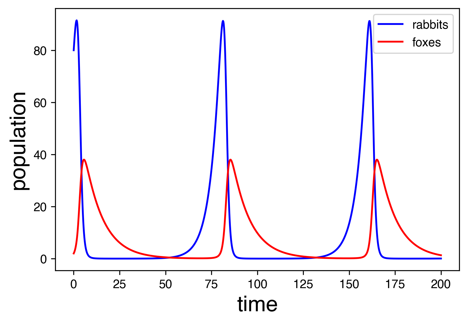
Fig. 9.2 Periodic time evolution of the population of rabbits and foxes.

The solution is periodic. This can be illustrated better by plotting \(f\) against \(r\). The animation below shows this (this kind of plot is called a phase plot). Note that a numerical solution now requires a better solving technique than our simple loop that increments time with a time step \(dt\). A so-called higher order scheme (Runga-Kutta 45) is employed. Low order schemes introduce too large errors and the solution does not look period. In other words: the phase plot is not a closed trajectory.

Fig. 9.3 Phase plot of the rabbit-fox prey-predator model. The red dot shows the population at different times. Note that the number of rabbits quickly increases when there are very few foxes. However, at some point the number of foxes also goes up and soon they start reducing the rabbits, while increasing in numbers themselves. That is not sustainable and when the number of rabbits is brought down substantially, also the number of foxes decreases, until both are almost extinct and the cycle repeats.

9.1.2. Wilberforce Oscillator

As a second example we look at the Wilberforce pendulum. This is a spring, suspended vertically, to which a weight is fixed at the free end. The weight can go up and down but also rotate in a horizontal plane. A sketch is given below.

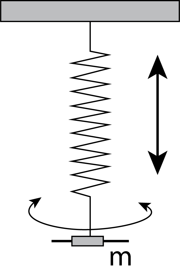
Fig. 9.4 Wilberforce pendulum.

Image that we pull \(m\) a little down and let go. The spring will try to restore the position of the mass to the equilibrium position it was in prior to us pulling \(m\) down. Consequently, \(m\) will start oscillating in the vertical direction. However, something peculiar happens: the mass \(m\) also starts to rotate (around the vertical axis). And also this rotation turns out to be a back and forth oscillation. But that is not all: the two oscillations are coupled: they feed each other. If the vertical oscillation is at a maximum amplitude, the rotational motion is almost zero and vice-versa.

Click Wilberforce to see a youtube video of this oscillator.

The system can be modeled with simple means. We will just postulate them. Later on, we will see where the terms come from.
First, we note that the mass has kinetic energy, in two forms: due to the vertical motion (\(\frac{1}{2}m\dot{z}^2\)) and due to the rotational motion (\(\frac{1}{2}I\dot{\theta}^2\)). Don’t worry about the exact meaning for now.
Second, the mass has potential energy. We will ignore gravity (and pretend we do this experiment in SpaceLab). A potential energy is associated with the vertical motion and is the spring energy: \(V_z = \frac{1}{2}kz^2\), with \(z\) the vertical position of the mass with respect to the equilibrium position, which we took as \(z=0\). \(k\) is the spring constant and represents the strength of the spring. We will come back to this later.
Then, we have potential energy associated with the rotation: \(V_\theta = \frac{1}{2} \delta \theta^2\). \(\theta\) represent the rotation angle, where we have taken \(\theta = 0\) in the equilibrium position. \(\delta\) is the torsional spring constant: it represents how strongly the spring tries to push back against rotation.
Finally, the vertical position and the rotation influence each other. That can be understood by realizing that if you shorten the spring, the spring material has to go somewhere. It can not only change its vertical length as that would mean that the total length of the spring would reduce. But that would compress the spring material and that is not possible for solid material (unless you apply incredibly large forces). The spring just increases its number of windings a bit. But that implies rotation. Similarly, if we only rotate the spring, it will try to adjust its length. As a consequence, there is also a potential energy involved in the influencing of \(z\) and \(\theta\) of each other. It can be modeled as \(V_{z\theta} = \epsilon z \theta\).

If we ignore friction, then we have a system that can be described in terms of kinetic and potential energy:

\[\frac{1}{2}m\dot{z}^2 + \frac{1}{2}I\dot{\theta}^2 + \frac{1}{2}kz^2 + \frac{1}{2}\delta \theta^2 + \epsilon z \theta = E_0 \]

From this, we can find ‘N2’, the equation of motion:

\[\begin{split}\begin{split} m\ddot{z} &= -kz - \epsilon \theta \\ I\ddot{\theta} &= -\delta \theta - \epsilon z \end{split}\end{split}\]

Don’t worry, if you don’t follow this. The point here is, that we have a coupled system of two oscillators. They can be solved numerically with a simple approach: instead of writing \(m\ddot{z}\) we can also use that \(v = \dot{z}\). With this, we can write the above system of 2 second-order differential equations as 4 first-order ones. That may sound like complicating stuff, but it actually does the opposite. Thus, we are going to try and numerically solve

\[\begin{split}\begin{split} \frac{dz}{dt} &= v \\ m\frac{dv}{dt} &= -kz - \epsilon \theta \\ \frac{d\theta}{dt} &= \omega \\ I\frac{d\omega}{dt} &= -\delta \theta - \epsilon z \end{split}\end{split}\]

We could use the simple scheme we have employed in Chapter 3. This updates the 4 unknowns after every time step, i.e. \(z(t+dt) = z(t) + v(t)dt\) and \(v(t+dt) = v(t) -\frac{k}{m} z(t) dt - \frac{\epsilon}{I} \theta (t) dt\) and likewise for \(\theta\) and \(\omega\).
In the figure below \(z(t)\) and \(\theta (t)\) are shown using such a simple numerical scheme.

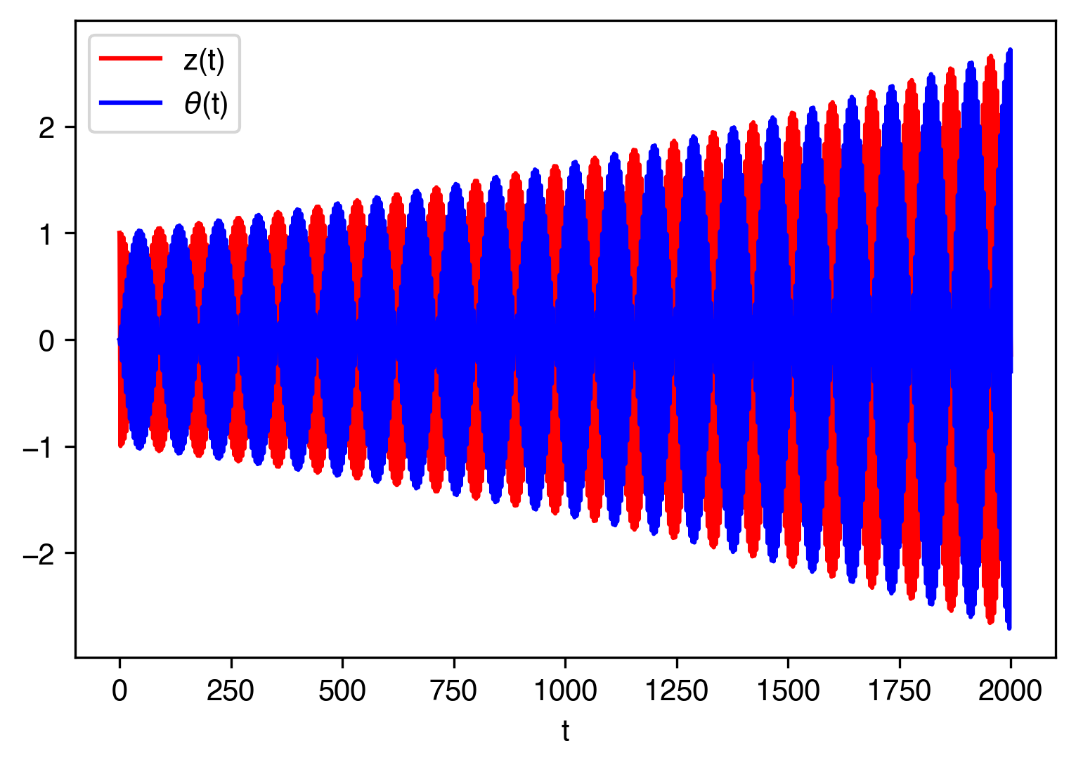
Fig. 9.5 Numerical solution of the Wilberforce pendulum using a (too) simple numerical method.

We indeed see the oscillating motion and that the vertical oscillation changes over to rotation and back again.

But there is something really disturbing: the amplitude of our oscillation is increasing and it seems to do so for every cycle. That cannot be true: it violates energy conservation. What did we do wrong? Well, our numerical method is just not good enough. If we use again a higher order method, we obtain the results in the figure below.

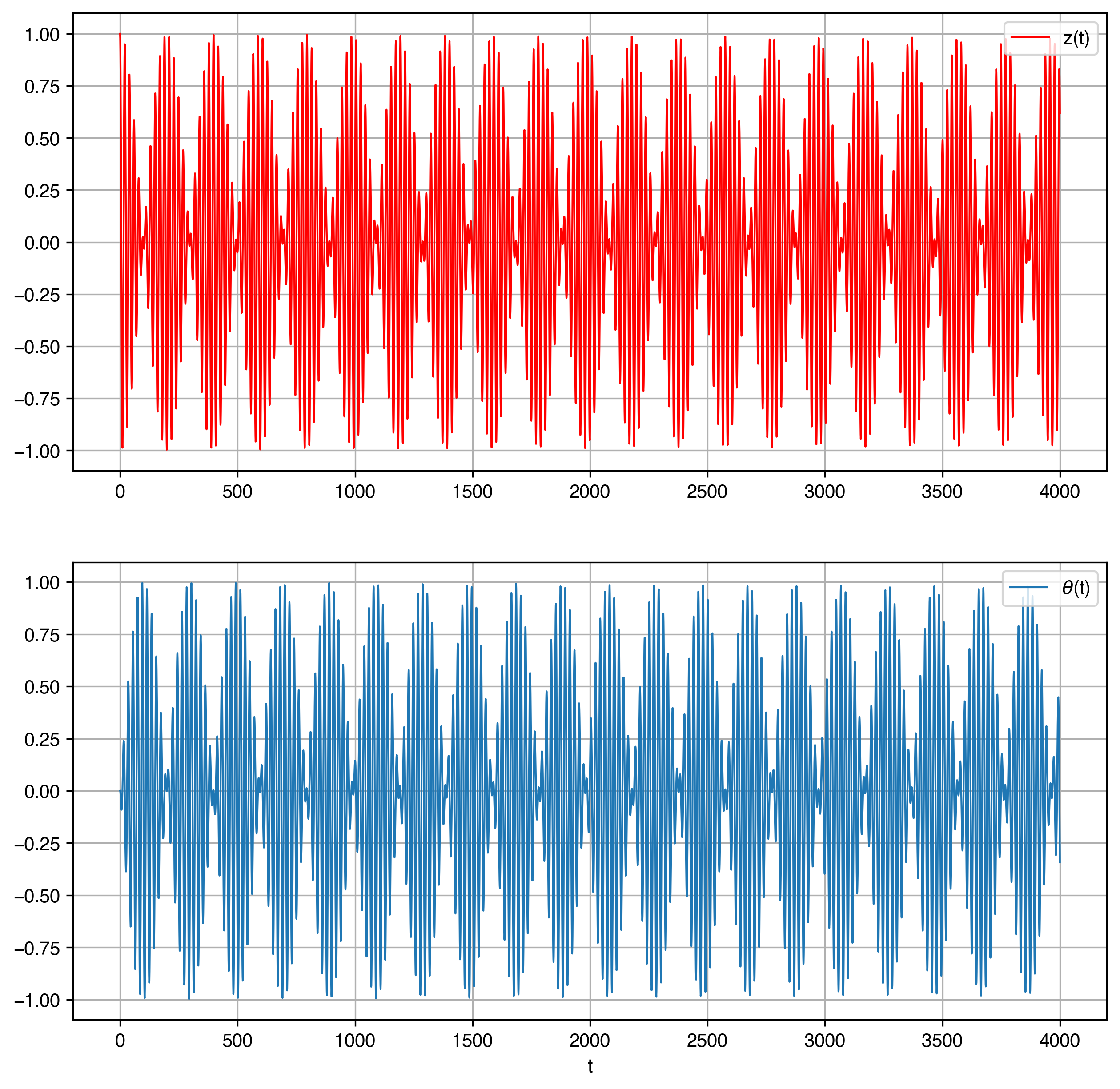
Fig. 9.6 Numerical solution of the Wilberforce pendulum using a higher-order numerical method.

Now the amplitude of the oscillations stays nicely constant, obeying conservation of energy.

In the figure below a small animation can be seen: the marker in both graphs shows \(z\) and \(\theta\) at the same time instant.

Fig. 9.7 Animation of the Wilberforce pendulum using a higher-order numerical method.

The Wilberforce pendulum is clearly periodic. Moreover, it is an oscillation as there is back and forth motion around an equilibrium.

But, it does give us a big warning: (numerical) solutions always have to be assessed against the features and principles of the problem at hand. In this case, our first numerical solution could not be right: it violated energy conservation. We were able, right from the start, to formulate the problem in terms of energy. Since we only had kinetic energy and potential energy we knew up front that the motion must be bounded!
That is why, we need a thorough understanding of physics. It is not sufficient to have the equations and put them in a ‘solver’. It is the job of a physicist to understand and assess models, outcomes, etc against the laws of physics. Hence, we will dive into oscillations, starting from the beginning.

9.2. Harmonic Oscillation - archetype: Mass-Spring

The archetype of an oscillation is the mass-spring system. It is the simplest version (simpler than the pendulum as we will see). And it can be recognized in many systems. We consider the following: a mass is attached to the end of a spring. The other end of the spring is fixed to a wall. The mass can only move in one direction: the \(x\)-direction. The spring has a natural or rest length \(l_0\). That is the length of the spring if no force is acting on it. If we pull the spring, it will exert a force that is proportional to the increase in length. Moreover, it is pointing in the direction opposite to the lengthening. In formula:

\[F_v = - k (l - l_0 ) = -k \Delta l \]

This is shown in the figure below.

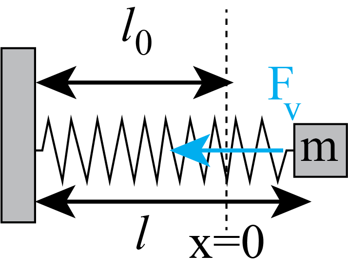
Fig. 9.8 Mass-spring system: archetype of a (harmonic) oscillation.

The response of the spring is to exert a force on \(m\) proportional to its elongation (which may be negative). It is clearly a restoring force: no matter what we do pulling or pushing, the spring will always counteract.

It is not difficult to set up N2 for the mass-spring. There is only one force and the system is 1-dimensional. If we define the origin at the position of the mass when the spring is at its rest length, then \(\Delta l\) - the elongation of the spring becomes \(x\), the coordinate of the mass \(m\). Thus N2 reads as:

\[ m\ddot{x} = -kx \]

Or

\[ m\ddot{x} + kx = 0 \]

To solve this, we need two initial condition. Let’s take \(t=0: x(0) = x_0, v(0) = 0\). We need to find a function \(x(t)\) that upon differentiating it twice, spits itself back but with an opposite sign. We do know two functions that do so: \(x(t) = \sin ( \omega_0 t)\) and \(x(t) = \cos ( \omega_0 t)\). Thus, the general solution of the above equation is known.

    Harmonic Oscillator:

\[ m\ddot{x} + kx = 0 \Leftrightarrow x(t) = A \sin \omega_0 t + B \cos \omega_0 t\]

If we insert the general solution, we find

\[\omega_0^2 = \frac{k}{m} \]

This is called the natural frequency of the oscillator. Note, that it does not depend on the initial conditions. No matter what, the mass will always oscillate with this frequency.

It does make sense that the frequency is inversely proportional to m: we expect that a heavy object will respond slow to a force. Similarly, if the spring is strong, that is, has a high spring constant \(k\), it will move the mass around quickly.

If we substitute the initial condition, we can completely solve the motion of the mass:

\[\begin{split}\begin{split} &m\ddot{x} + kx = 0 \Rightarrow x(t) = A \sin \omega_0 t + B \cos \omega_0 t \Rightarrow \\ \\ &\begin{cases} v(0 = \dot{x}(0) = 0 \rightarrow A \omega_0 \underbrace{\cos 0}_{=1} - B \omega_0 \underbrace{\sin 0}_{=0} = 0 \rightarrow A = 0 \\ x(0) = \Delta x \rightarrow B \cos 0 = \Delta x \end{cases} \\ \\ &\Rightarrow x(t) = \Delta x \cos \sqrt{\frac{k}{m}} t \end{split}\end{split}\]

A system is called a harmonic oscillator if and only if it obeys \(m\ddot{x} + kx = 0\). You will find them in almost every branch of science and engineering. The reason why will become apparent in a moment.

9.2.1. Potential energy of a spring

In the above, we have formulated the mass-spring system in terms of Newton’s second law. We can, however, also cast it in the form of energy. The force of the spring is conservative. We can easily prove that by finding the associated potential energy: \(F_v = -\frac{dV}{dx}\).
Since \(F_v = -kx\) we need to find a function \(V(x)\) that satisfies \(\frac{dV}{dx} = kx\). Let’s do it:

\[ \frac{dV}{dx} = kx \Rightarrow V(x) = \frac{1}{2} x^2 + C \]

We have the freedom to decide ourselves where we want the potential energy to be zero. Note: \(V\) is quadratic.

It does make sense, to set the minimum of the potential energy such that if the mass is at the equilibrium position, the potential energy is zero, that is - take \(C=0\):

\[ V(x) = \frac{1}{2}kx^2 \]

Thus the mass-spring system can also be described by

\[ \frac{1}{2}mv^2 + \frac{1}{2}kx^2 = E_0 \]

So, an other way of stating what a harmonic oscillator is: it is a system that obeys the above energy equation.

9.3. Behavior around an equilibrium point and harmonic oscillators

Now we will go back to paragraph 5.5.1, where we discussed the Taylor series expansion of the function \(f(x)\):

\[ f(x) \approx f(x_0) + \frac{1}{1!} f'(x_0) (x-x_0 ) + \frac{1}{2!} f''(x_0) (x-x_0)^2 + \mathcal{O}(x^3) \]

We will apply it to a potential energy \(V(x)\) of some system. We assume that the system has a stable equilibrium point at \(x=x_0\), that is \(\left [ \frac{dV}{dx} \right ]_{x=x_0} = 0\) and \(\left [ \frac{d^2V}{dx^2} \right ]_{x=x_0} > 0\).
Thus, we can expand the potential around the stable point as follows:

\[ V(x) \approx V(x_0) +\frac{1}{1!} \underbrace{\left [ \frac{dV}{dx} \right ]_{x=x_0}}_{=0} (x-x_0 ) + \frac{1}{2!} \underbrace{\left [ \frac{d^2V}{dx^2} \right ]_{x=x_0}}_{=k} (x-x_0 )^2 + \mathcal{O} \left [ (x-x_0 )^3 \right ] \]

If we plug this in, in the energy equation and cut off after the quadratic term, we find

\[\frac{1}{2}mv^2 + V(x_0) +\frac{1}{2} \underbrace{\left [ \frac{d^2V}{dx^2} \right ]_{x=x_0}}_{=k} (x-x_0 )^2 = E_0 \]

or shortened by the abbreviation \(\left [ \frac{d^2V}{dx^2} \right ]_{x=x_0} = k\)

\[\frac{1}{2}mv^2 + V(x_0) +\frac{1}{2}k ((x-x_0)^2 = E_0\]

Move the constant \(V(x_0)\) to the right hand side and change coordinate \( s \equiv x-x_0 \rightarrow \dot{s} = \dot{x} = v\). This gives us:

\[ \frac{1}{2}m\dot{s}^2 + \frac{1}{2}ks^2 = C \]

The harmonic oscillator!!! No wonder we find harmonic oscillators ‘everywhere’. Any system that has a stable equilibrium point (i.e. with a positive second derivative of its potential) will start to oscillated as a harmonic oscillator if we push it a little bit out of its equilibrium position. Doesn’t matter how \(V(x)\) exactly is. It doesn’t have to be quadratic in \(x\). But it will be pretty close to that, if we stay close enough to the equilibrium point. Hence, any small natural kick, any small amount noise will push a system out of its stable equilibrium point into an harmonic oscillating motion with a given, natural frequency given by \(\omega_0^2 = \frac{\left [ \frac{d^2V}{dx^2} \right ]_{x=x_0}}{m}\).

9.4. Examples of Harmonic Oscillators

9.4.1. Torsion Pendulum

We take a straight metal wire. Suspend one end at the ceiling and attach a disc of radius \(R\) and mass \(m\) at the other end.

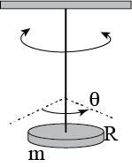
Fig. 9.9 Torsion Pendulum.

The disk can rotate about a vertical axis. We call the rotation angle \(\theta\). The equilibrium position is \(\theta = 0\). If we rotate the disc over a small angle, the wire will resist and apply a torque \(\Gamma\) on the disc trying to rotate the disc back to its equilibrium position, for which the torque, obviously is zero.

For small angles, the torque is proportional to the rotation angle and -of course -working in the direction opposite of the rotated angle. We can set up an angular momentum balance and find that it reads as:

\[ I \frac{d^2\theta}{dt^2} = - k_t \theta \]

In this equation, \(I = \frac{1}{2}mR^2\) is the moment of inertia of the disc (we will discuss rotations of solid bodies in a separate chapter) and \(k_t\) is the torsion constant of the wire. Don’t worry about the exact meaning of the terms in the equation. For now, we focus on the equation itself:

\[ I \frac{d^2\theta}{dt^2} + k_t \theta = 0 \Rightarrow \theta (t) = A \sin \omega_0 t + B \cos \omega_0 t\]

The torsion pendulum is an harmonic oscillator, \(\omega_0^2 = \frac{k_t}{I}\), completely analogous to the archetype, mass-spring. Obviously, we thus can also write this in terms of energy:

\[ \frac{1}{2} I \omega^2 + \frac{1}{2}k_t \theta^2 = E_0 \]

with \(\omega \equiv \frac{d\theta}{dt}\), the angular velocity.

9.4.2. L-C circuit

In Electronics alternating current (AC) circuits are building blocks of many complex systems. One of these is the L-C circuit, in which an inductor, \(L\), and a capacitor, \(C\), are in series coupled. See Fig. 9.10.

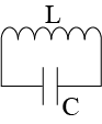
Fig. 9.10 L-C circuit.

We could charge the capacitor and then close the circuit. What would happen? The capacitor will try to discharge via the inductor. Hence a current, \(I\), starts flowing. In response the inductor builds up a potential difference that is directly proportional to the rate of change of the current through the inductor.

Basic electronics shows that the voltage over the capacitor is coupled to the charge, \(Q_C\) of the capacitor according to: \(V_C = \frac{Q_C}{C}\). For the inductor we have: \( V_L = L \frac{dI_L}{dt}\).

According to Kirchhoff’s laws the current through both elements must be the same: \(I_C = I_L\) and the sum of the voltages across them must be equal to zero: \(V_c + V_L = 0\). If we put everything together, we get - using \(I_C = \frac{dQ_c}{dt}\):

\[\begin{split}\begin{split} V_L + V_C &= 0 \Rightarrow \\ \frac{dV_L}{dt} + \frac{dV_C}{dt} &= 0 \Rightarrow \\ L \frac{d^2 I}{dt^2} + \frac{1}{C}I &= 0 \Rightarrow \\ \frac{d^2I}{dt^2} + \frac{1}{LC} I &= 0 \text{ Harmonic Oscillator!!!} \end{split}\end{split}\]

As we see, this LC-circuit will start to oscillate. In the animation below the current through the circuit and the voltage across the inductor are shown for \(C = 1 \mu F\) and \(L = 1 \mu H\).

Fig. 9.11 Harmonic oscillation of an LC-circuit.

9.4.3. Musical Instruments

Musical instruments produce sound waves. In many cases they do that via vibrating strings, like the guitar, the violin, harp or piano. The strings of these instruments are displaced out of their equilibrium position. Due to the tension in these strings, there is a restoring force that is proportional to the displacement. Consequently, the string will start to oscillate in an harmonic way.

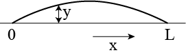
Fig. 9.12 Vibrating string.

If we call the coordinate along the string \(x\), then the displacement of the string with respect to its equilibrium \(y\) is a function of \(x\): \(y = y(x)\). Obviously, the displacement is also a function of time, so we need to consider \(y(x,t)\) making it a much more complicated problem than our mass-spring.

We will not go into the details, but be satisfied with postulating the equation of motion of the string:

\[ \mu \frac{\partial^2 y}{\partial t^2} = T \frac{\partial^2 y}{\partial x^2}\]

with \(\mu\) the mass of the string per unit length, i.e. \(\mu = \frac{m}{L}\) and \(T\) the tension in the string.

The above equation is called the wave equation and although it looks and is much more complicated than the mass-spring harmonic equation, it has quite some resemblances. For instance, the frequency with which the string will oscillate is given by multiples of the so-called ground-frequency, \(f_0 = \frac{1}{2L} \sqrt{\frac{T}{\mu}}\). Moreover, each point of the string will oscillate in a \(\sin\) and \(\cos\) way. The string has the tendency to vibrate in a sinusoidal way: both in space and time. Standing waves will form on the string, with a frequency that is an integer multiple of the ground-frequency

Fig. 9.13 Fundamental modes of a vibrating string.

Not only strings, but also beams will exhibit this behavior, well-known example: a tuning fork.

9.5. The pendulum

Another example of oscillatory motion is the pendulum. In its most simple form it is a point-mass \(m\), attached to a massless rod of length \(L\). The rod is fixed to a pivotal point that allows it to swing freely.

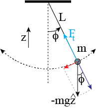
Fig. 9.14 Sketch of the forces on a pendulum.

On the mass, gravity is acting vertically downwards. Also the rod exerts a force on the mass. This force is always parallel to the rod and points to the pivotal point. It is the response of the rod to the component of gravity parallel to the rod (the dark blue arrow in Fig. 9.14). It is good to realize, that this force makes sure that the distance from \(m\) to the pivotal point is always \(L\). In other words, this force is a consequence of the fixed length \(L\) of the rod. It is the physics translation of the constraint: \(L\) is constant.

9.5.1. N2 for the pendulum: Equation of motion via N2

We will set up Newton’s second Law for \(m\).

\[ m\frac{d\vec{v}}{dt} = -mg\hat{z} + \vec{F}_t \]

As stated above, the dark blue, parallel part of gravity is balanced by a tensional force in the rod. So, we don’t need to worry about motion of \(m\) parallel to the rod. That leaves us with the direction perpendicular of the rod. In that direction only the red arrow works on \(m\).

We recognize that the blue and red directions actually are best described in polar coordinates. The two blue arrows, \(F_t\) and \(F_{g//}\) work in the \(\hat{r}\) direction and make sure that the component of the acceleration in this direction is zero.

The other direction with coordinate \(\phi\) and unit vector \(\hat{\phi}\) has only the red, perpendicular component of gravity. This component points in the negative direction of \(\phi\) and is equal to \(-mg \sin \phi \text{ }\hat{\phi}\). The velocity component in the \(\phi\) direction is \(v_\phi = r\frac{d\phi}{dt}\). In the case of the pendulum, the \(r\) coordinate is always \(L\), the length of the rod. Thus for the \(\phi\)-direction we get:

\[ m L \frac{d^2 \phi}{dt^2} = -mg \sin \phi \]

Or rewritten

\[ m L \frac{d^2 \phi}{dt^2} + mg \sin \phi =0 \]

We do know from experience that the pendulum will swing back and forth in a periodic way. However, as we see from the above equation of motion: it is not a harmonic oscillator. The term with the sin prevents that.

But, for small values of the angle \(\phi\), that is for small oscillations around the stable equilibrium \(\phi_{eq} = 0\), we can approximate the sinus via a Taylor series and write:

\[\begin{split} \begin{split} \phi \ll 1 \Rightarrow\sin \phi &\approx \sin 0 + \frac{1}{1!} \cos 0 \: \phi - \frac{1}{2!} \sin 0 \: \phi^2 + ... \\ &\approx \phi \end{split} \end{split}\]

Thus, within this approximation we can write for the equation of motion of the pendulum:

\[m L \frac{d^2 \phi}{dt^2} + mg \phi =0 \Rightarrow \frac{d^2 \phi}{dt^2} + \frac{g}{L} \phi =0\]

and that describes a harmonic oscillator.

Thus we conclude that for small amplitudes of the oscillation, the pendulum is an harmonic oscillator and swings in a sin or cos way back and forth. Moreover, the oscillation has a frequency

\[ \omega_{pendulum} = \sqrt{\frac{g}{L}}\]

Further, note that under this assumption, the period of the pendulum does not depend on the amplitude of the oscillation, nor does it depend on the mass. This was already noted by Galileo Galilei.

9.5.2. N2 for the pendulum: Equation of motion via Angular Momentum

Before we continue with the analysis of the pendulum, we will derive the equation of motion also via angular momentum considerations. On \(m\) gravity exerts a torque: \(\Gamma = \vec{r} \times \vec{F}_g = -Lmg \sin \phi \: \hat{\phi} \). The force from the rod is parallel to the position vector and does not exert a torque on \(m\). The angular momentum of \(m\) is given by \(\vec{L} = \vec{r} \times \vec{p} = mL^2\frac{d\phi}{dt}\hat{\phi}\).

Thus N2 for angular momentum gives us:

\[ \frac{d\vec{L}}{dt} = \vec{\Gamma} \Rightarrow mL^2\frac{d^2\phi}{dt^2} = -Lmg \sin \phi\]

Thus, angular momentum leads to the same equation of motion.

9.5.3. The Pendulum via energy conservation

Alternatively, we can also use energy conservation to derive the equation governing the motion of the pendulum. There are, as discussed above, two forces acting on \(m\). The first one is gravity, which is a conservative force with associated potential energy. We can write for this case \(V_g = mgz\), taking \(V_g (z=0) = 0\).

The second one is the force from the rod. But this one always acts perpendicular to the motion of \(m\). Hence, it does not do any work and, thus, we don’t need to worry about an associate potential.

We conclude that for the pendulum it holds:

\[ \frac{1}{2}mv^2 + mgz = E_0 \]

To solve this, we use -like above- polar coordinates. Notice that \(v_r = 0\) as the rod has a fixed length. Furthermore, the height of the mass above \(z=0\) is, in terms of \(\phi\): \(L - L\cos\phi\), see Fig. 9.15.

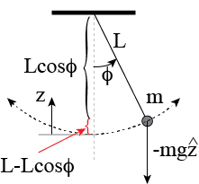
Fig. 9.15 Potential energy of a pendulum.

Thus, our energy equation reads as:

\[\frac{1}{2}m v_\phi^2 + mgL \left (1 - \cos \phi \right ) = E_0 \]

or

\[\frac{1}{2}m v_\phi^2 - mgL \cos \phi = E_0 - mgL \]

Take the time-derivative and use \(v_\phi = L\frac{d\phi}{dt}\) and we get

\[\begin{split} \begin{split} mv_\phi \frac{dv_\phi}{dt} + mgL \sin \phi \frac{d\phi}{dt} &= 0 \Rightarrow \\ mL \frac{d\phi}{dt} \frac{d}{dt} \left ( L \frac{d\phi}{dt} \right ) + mgL \sin \phi \frac{d\phi}{dt} &= 0 \Rightarrow \\ \frac{d^2\phi}{dt^2} + \frac{g}{L} \sin \phi &= 0 \end{split} \end{split}\]

And we have recovered the same equation of motion.

9.5.4. Pendulum for not so small angles

In the above we have frequently used the approximation \(\sin \phi \approx \phi \) for \(\phi \ll 1\). What about the general case? Then we need to solve

\[\begin{split} \begin{split} \frac{d^2\phi}{dt^2} + \frac{g}{L} \sin \phi &= 0 \\ \text{ with i.c. } \phi(0) = \phi_0 \text{ and } \frac{d\phi}{dt} = \dot{\phi}_0 \end{split} \end{split}\]

This equation is much more difficult to solve analytically and we will, therefore, use a numerical approach here. The animation below compares the motion of the pendulum numerically simulated to that of the pendulum when using the small amplitude approximation.

The animation shows: a green mass, that is the pendulum with a (fixed) small amplitude in the approximation \(\sin \phi = \phi\). The blue one uses the same approximation even though \(\phi\) is not small. Notice, that blue and green oscillate with exactly the same frequency. This is, of course, trivial as they obey the same harmonic oscillation equation and thus have the same frequency.

The red mass, on the other hand obeys the equation of motion of the pendulum leaving the term with \(\sin \phi\). It is clear that the real pendulum (i.e. the red one) does not have the same frequency as the others. Moreover, its time trace (left part of the figure) is clearly not a true sinus.

Fig. 9.16 Animation of the pendulum: red is the true pendulum, blue the small angle approximation applied to a large angle case and green the small angle approximation for a small angle.

In the widget below, you can vary the initial angle and observe that indeed for a small angle the red mass and the other two follow the same trajectory. But if you increase the initial angle, the red mass behaves differently: it oscillates slower and the time trace of angle as a function of time is no longer sinusoidal.

Or open the widget full screen

9.6. The damped harmonic oscillator

In the above, no friction of any form has been considered. However, in many practical cases friction will be present. For moving objects friction frequently depends on the velocity: the higher the velocity, the higher the frictional force. We will here consider the simples version: a friction force that is directly proportional to the velocity: \(F_f = -b v\) with \(b\) a positive constant. Thus, we need to add an additional force to our harmonic oscillator:

\[ m\ddot{x} = -k x - b \dot{x} \]

or bringing all terms to the left hand side:

\[ m\ddot{x} + b \dot{x} + kx = 0 \]

To solve this equation, it is easier not to try to look directly for sinus and cosins, but use the complex notation.

Intermezzo: complex exponential and sin, cos

In the 18\(^{th}\) century, the study of complex numbers, i.e. \(i = \sqrt{-1}\), revealed a surprising connection between the exponential function and trigonometry. It was Leonhard Euler (1707-1783) who derived:

\[e^{ix} = \cos x + i \sin x \]

If you want to understand this a bit further, write down the Taylor expansion of all three functions. By realizing that \(i^2 = -1, i^3 = i^2 i = -i\), etc. You will see that Euler was right.

We can use the above equation to write \(\sin x\) and \(\cos x\) as exponential functions:

\[\begin{split}\begin{split} \sin x & = \frac{e^{ix} - e^{-ix}}{2i} \\ \cos x & = \frac{e^{ix} + e^{-ix}}{2} \end{split} \end{split}\]

And we can also state that the real part of \(e^{ix}\) is equal to \(\cos x\) and the imaginary part to \(\sin x\).

The above turns out to be extremely useful in solving differential equations. For instance, rather than trying \(\sin\) and \(\cos\) as solutions for the harmonic equation \(m\ddot{x} + kx = 0\), we could try \(e^{i\omega t}\) (please note: x in the first part of this intermezzo is just a real number, whereas now x is the amplitude of the oscillator and is a function of \(t\)):

\[\begin{split} m\ddot{x} + kx = 0 \Rightarrow \\ m \frac{d^2 Ae^{i\omega t}}{dt^2 }+ k A e^{i\omega t} = 0 \Rightarrow\\ Am (i\omega)^2 e^{i\omega t} + Ak e^{i\omega t} = 0 \Rightarrow \\ Ae^{i\omega t} \left ( -m\omega^2 +k \right ) = 0 \;\;\;\;\forall t \end{split}\]

Thus we conclude that if \(Ae^{i\omega t}\) is a solution of the harmonic equation, then \(\omega^2 = \frac{k}{m}\). So, with that condition, \(Ae^{i\omega t}\) is a solution with \(A\) an integration constant that will be fixed by proper initial conditions.

But let’s be careful: the harmonic oscillator is governed by a second order differential equation, that is we have differentiated twice with respect to time. Thus we need to integrate also twice, leaving us with 2 rather than 1 integration constant. Hence, we have not found the general solution, yet.

That can be easily cured: if \(Ae^{i\omega t}\) is a solution, then \(Be^{-i\omega t}\) is one as well. And here is our second solution, with the same condition for \(\omega\). And our general solution is

\[x(t) = Ae^{i\omega t} + Be^{-i\omega t} \]

Note that \(A\) and \(B\) are complex numbers and thus, we can always rewrite this equation back into \(\sin (\omega t)\) and \(\cos (\omega t)\). But in most cases we don’t worry about that. We are interested in the ‘rule’ for \(\omega\) and once we have that, we can write our solution straightaway as \(x(t) = C\cos (\omega t) + D \sin (\omega t)\).

Let’s use this for the damped harmonic oscillator:

\[m \ddot{x} + b \dot{x} + kx = 0 \]

Try \(x(t) =A e^{i \omega t}\).

\[\begin{split} \Rightarrow Ae^{i\omega t} \left ( -\omega^2 m + i \omega b + k \right ) = 0 \;\;\;\;\; \forall t \Rightarrow\\ \omega^2 m - i \omega b - k = 0 \Rightarrow \\ \omega_{+,-} = \frac{+ib \pm \sqrt{-b^2+4mk}}{2m} \end{split}\]

We immediately have our two solutions: one with the \(+\)sign, the other with \(-\)sign:

\[x(t) = A e^{i\omega_+ t} + B e^{i\omega_- t} \]

with both \(\omega\)’s complex numbers.

Alternatively, we could have started with \(x(t) = e^{\lambda t}\), but allowing \(\lambda\) to be a complex number. This somewhat easier and as we have seen above, \(\omega\) is a complex number (\(D = -b^2+4mk\) can be negative). This will gives us:

\[ m\lambda^2 + b\lambda + k = 0 \Rightarrow \lambda_{+,-} = \frac{-b \pm \sqrt{b^2 - 4mk}}{2m} \]

We see, that \(\lambda\) always has a negative real part. That makes sense: the negative real part shows that the solution is damped.

Our solution to the damped harmonic oscillator is thus:

\[ x(t) = A e^{\lambda_+ t} + B e^{\lambda_- t} \]

The general solution of the (linearly) damped harmonic oscillator is:

\[\begin{split} m\ddot{x} + b \dot{x} + kx = 0 \Rightarrow \\ \; \\ x(t) = A e^{\lambda_+ t} + B e^{\lambda_- t} \\ \; \\ \text{with} \\ \; \\ \lambda_{+,-} = \frac{-b \pm \sqrt{b^2 - 4mk}}{2m} \end{split}\]

We will investigate various cases.

Case 1 \(D = b^2 - 4mk \lt 0\)

In this case, the square root in \(\lambda\) is imaginary and we can write it as \(i\sqrt{4mk - b^2}\). This gives us for the two possibilities of \(\lambda\)

\[\begin{split} \lambda_+ = -\frac{b}{2m} + i \sqrt{\frac{k}{m} - \frac{b^2}{4m^2}} \\ \;\\ \lambda_- = -\frac{b}{2m} - i \sqrt{\frac{k}{m} - \frac{b^2}{4m^2}} \end{split}\]

Both have the same real part: \(-\frac{b}{2m}\) showing that both solutions are damped (with the same factor!). Moreover, the imaginary parts are equal, apart from the sign which we also had in the undamped case. We will write the imaginary part as \(\omega\) (that is without the subscript 0 we used for the undamped case).

So, our solution reads as:

\[\begin{split} x(t) = \underbrace{\left ( A e^{i\omega t} + B e^{-i\omega t} \right )}_{sinusoidal \; oscillation} \underbrace{e^{-\frac{b}{2m} t}}_{exponential damping} \; \\ \; \\ with \\ \; \\ \omega \equiv \sqrt{\frac{k}{m} - \frac{b^2}{4m^2}} \lt \sqrt{\frac{k}{m}} = \omega_0 \end{split}\]

Conclusion: the damped oscillator oscillates with a smaller frequency than the undamped one and it amplitude decreases over time. The later is of course to be expected due to friction: sooner or later friction has dissipated all the kinetic & potential energy.

Case 2 \(D = b^2 - 4mk = 0\) For this specific combination of \(b, k, m\) we see that the frequency of the oscillation is 0. In other words, the systems does not perform oscillations. Furthermore, our two values of \(\lambda\) are now equal. Consequently the general solution that we presented is no longer complete (we now only have one integration constant, or only one independent function if you prefer.) We need a second one and that turns out to be of the form \(t e^{\lambda t}\). You can verify that by substituting it in the equation of motion for the damped case.

Thus we have know:

\[\begin{split} D = b^2 - 4mk = 0 \Rightarrow \\ \;\\ x(t) = \left ( A + B t \right ) e^{-\frac{b}{2m} t} \end{split}\]

Case 3 \(D = b^2 - 4mk \gt 0\) Again, there is no imaginary part in \(\lambda\), so no oscillations. But we do have two different values for \(\lambda\) and thus our original general solution is still valid:

\[ x(t) = A e^{\frac{-b + \sqrt{b^2 - 4mk}}{2m}t} + Be^{\frac{-b - \sqrt{b^2 - 4mk}}{2m}t} \]

Note that \( -b + \sqrt{b^2 - 4mk} \lt 0 \). So, both terms are decreasing to zero: the motion comes to a stop as \(t \rightarrow \infty\).

Further, note that the first part (with \(A\)) has an exponent that is closer to zero than the one of the other part (with \(B\)). Thus the second part will decay faster and for sufficiently large \(t\), the solution behaves like \(A e^{\frac{-b + \sqrt{b^2 - 4mk}}{2m}t}\).

In the figure below, an example of case 1 and case 3 is shown together with the solution of case 2. We see, that case 2 is the one that decays fastest: it has the highest damping coefficient in its exponent. This is called critical damping. If you need to dampen unwanted oscillations: make sure you tune your damping parameter b such that \(b^2 - 4mk = 0\).

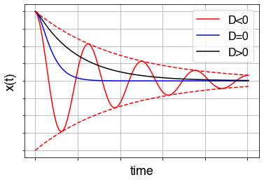
Fig. 9.17 Different cases for the damped harmonic oscillator.

9.6.1. Evolution of the damping

Here we will have a quick look how the damping is evolving, that is we look at the root of the characteristic equation

\[ \lambda_{1/2} =\frac{-b \pm \sqrt{b^2 - 4mk}}{2m} \]

and see how it evolves as a function of the damping \(b\) in the complex plane.

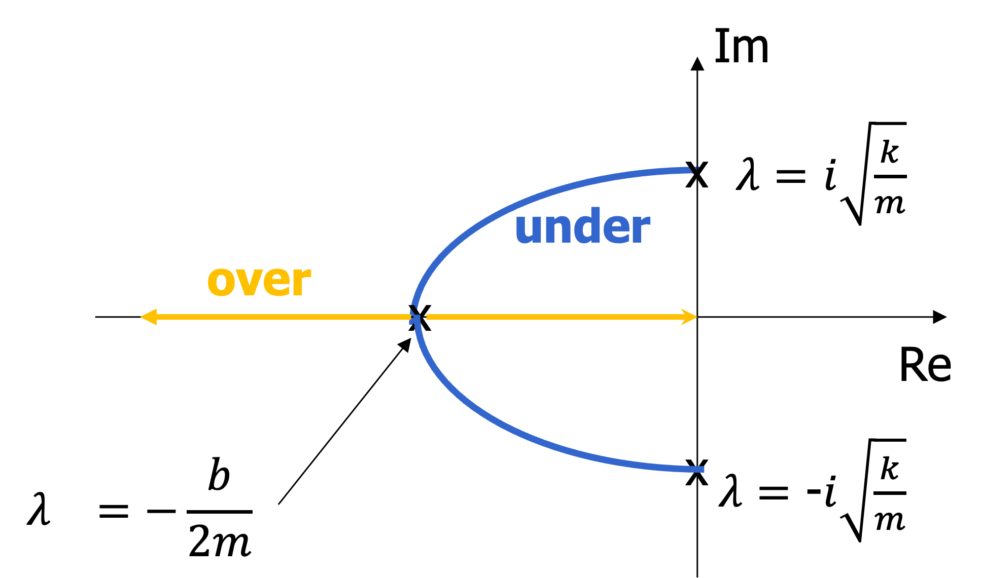
Fig. 9.18 Evolution of \(\lambda\) as a function of \(b\) in the complex plane.

This gives quickly a qualitative view on the different regimes of the damping. The root \(\lambda_{1/2}\) is in general complex. We start by looking at the value for roots \(\lambda_{1/2}\) as a function of the damping \(b\)

• No damping: \(b=0\). The root is pure imaginary \(\lambda_{1/2}=\pm i\sqrt{k/m}\) with two conjugate solutions on the imaginary axis. This gives pure oscillations.

• Some damping \(0<b<\sqrt{4mk}\). The root is complex, with real and imaginary part, the oscillation will damp out over time (shown in blue, underdamped regime).

• \(b^2=4mk\). The roots collapse into one pure real root \(\lambda=-b/2m\) (critically damped), no oscillation.

• Lots of damping \(b>\sqrt{4mk}\). The root splits into two real roots, no oscillations (shown in yellow, overdamped regime).

The root walks over the shown graph from \(b=0\) on the imaginary axis to \(b\to\infty\) over the blue and then yellow part of the graph. The yellow graph does not cross the imaginary axis.

From this plot you can directly see that the system is stable for \(b>0\), but unstable for \(b=0\) without the need to check the frequency that the system is driven with (for \(b=0\) driven with the resonance frequency results in an infinite amplitude - an instable system). How you can see that so quickly you will learn in the second year class Systems and Signals.

9.7. Driven Damped Harmonic Oscillator

Oscillators sometimes experience a driving force that can be periodic in itself. We will take here the case of a sinusoidal force with frequency \(\nu\). Once we understand this, forces consisting of more than one frequency (broader spectrum) can be understood using Fourier analysis (which you will learn about classes like Systems and Signals or Fourier Analysis in math). There you will also learn to treat this system in more detail analytically. Here we will stick to a simple driving force of the form \(F_{ext} = F_0 \sin (\nu t)\).

This gives for the equation of motion:

\[ m\ddot{x} +b\dot{x} +kx= F_0 \sin (\nu t) \]

with initial conditions: at \(t= 0\) the particle will have some position \(x_0\) and some velocity \(v_0\).

The solution of the driven damped harmonic oscillator equation of motion for the case \(D = b^2 - 4mk < 0\) is:

\[ x(t) = A e^{- \frac{b}{2m} t} \sin \left ( \sqrt{\frac{k}{m} - \frac{b^2}{4m^2}} t+ \epsilon \right ) + x_{max} \sin \left ( \nu t + \alpha \right ) \]

With \(A\) and \(\epsilon\) determined by the initial conditions.

The two other parameters \(x_{max}\) and \(\alpha\) are fixed. We will give only the expression for \(x_{max}\):

\[ x_{max} = \frac{F_0}{\sqrt{\left ( \omega_0^2 - \nu^2 \right ) ^2 + \frac{b^2}{m^2} \nu^2}} \]

For \(t\to\infty\), the second part, i.e., the term from the driving force \(x_{max} \sin \left ( \nu t + \alpha \right )\), survives as the exponential decay will have damped the first term. The oscillation will have frequency \(\nu\) of the driving force. As can be seen, the amplitude of the motion is for longer times \(x_{max}\).

If the driving frequency \(\nu\sim\omega_0\), the amplitude increases strongly. Especially for small damping, i.e., small \(b\), the amplitude will increase to high values. This phenomenon is called resonance:

\[ \text{if } b \rightarrow 0 \text{ and } \nu \rightarrow \omega_0 \text{ then } x_{max} \rightarrow \infty \text{ resonance} \]

9.8. Coupled Oscillators

In this course we mostly only consider one oscillator, but of course there could be many that are coupled in one way or another. Already Christiaan Huygens considered them.

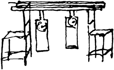
Fig. 9.19 Huygens experiment of weakly coupled pendula.

There are 2 pendula suspended from a common connection, which rests on two chairs. If you set the pendula in motion, they will be initially out of phase, i.e. the relative position of the pendula is different. But over time their motion synchronises! What has happend? Apparently the two pendula are connected, coupled, via the suspension and act on each other, they are not independent, but influence the motion of the other pendulum.

The video below shows a modern day version of this phenomena.

Video by Tetsuro Konishi at Physics Demo.

Here the pendula are coupled via the ground. This influence is called weak coupling. In this course we cannot treat this coupling mathematically, but in the second year course on Classical Mechanics you will learn to study systems like these.

9.9. Examples

1. Example of resonance: sound waves are exciting a glass. By changing the frequency of the sound waves to the resonance frequency, the glass starts oscillating with increasing amplitude until it finally breaks.

2. Driven harmonic oscillator with damping.

Or open the widget full screen

3. 1940: the Tacoma Narrows Bridge in the state Washington on the West coast of the USA is brought into resonance by the wind. The end result: click the movie to see it yourself.

4. Breaking a HDD hard disk with a song of Janet Jackson

Read here about this truly amazing piece of applied physics on a blog of Microsoft developer Raimond Chen.

5. Raman scattering.

If electromagnetic radiation interacts with a molecule to zero order, then the molecule does not vibrate or rotate. The radiation with field \(E(t)=E_0 \cos (2\pi \nu_0 t)\) then induces a dipole moment in the electron cloud of the molecule what will vibrate with the same frequency as the external field \(\nu_0\). This phenomena is called Rayleigh scattering

If the electrons in the molecule already oscillate with another frequency \(\nu_{vib}\), and the polarizability \(\alpha\) of the molecule depends on the distance \(R=R_0\cos (2\pi\nu_{vib}t)\) from the nuclei of the molecule, to first order the polarizability can be modeled as \(\alpha (R)= \alpha (R_0) + \alpha' (R-R_0)+ {\cal{O}} (R^2)\). The emitted field is therefore

\[\begin{split} \begin{array}{rcl} p(t) &=& \left [ \alpha(R_0)+\alpha' \cos (2\pi \nu_{vib}t) \right ] E_0 \cos(2\pi\nu_0 t)\\ &=& \alpha(R_0)E_0 \cos (2\pi\nu_0 t) \\ && +\frac{1}{2}\alpha' E_0 \left [ \cos(2\pi (\nu_0+\nu_{vib})t) + \cos(2\pi (\nu_0-\nu_{vib})t)\right ] \end{array} \end{split}\]

We see that next to the Rayleigh term \(\cos(2\pi\nu_0 t)\) two additional lines with frequency \(\nu_0\pm \nu_{vib}\) appear. These lines are called Raman lines. They are characteristic for the vibrational bands of the molecule present and are used to probe the presence of certain molecules in practice. NB: The line with frequency \(\nu_0+\nu_{vib}\) has higher energy than the incoming light. This line has a much smaller intensity than the \(\nu_0-\nu_{vib}\) line. To understand this you need to consider quantum mechanics and that the occupation of states is Boltzmann distributed (but this is beyond this example and you will learn more about this in the second and third year).

We hope that you see the similarity to the harmonic oscillator where the polarizability \(\alpha\) is modelled as a (restoring) force.

6. Second-harmonic generation

Of course the harmonic potential is only a first order approximation around an equilibrium. An example, for a non-linear force or anharmonic potential effect, is the generation of second-harmonic generation. If you shine high intensity light onto the electrons of a molecule, they are pushed out of equilibrium further and if the governing potential is anharmonic, the electric field response will not only include the incoming frequency \(\omega\) but also higher harmonics \(2\omega, 3\omega,\dots\), but with much lower intensity. That the emitted frequencies are occurring in integer multiple of the incident frequency can be understood either from quantization of light into photons (and the conservation of energy) or from Fourier analysis of the periodic motion of the electron.

7. Erasmus Bridge & singing cables.

The bridge in Rotterdam, but also others, suffer from long cables that the wind can put into resonance. Their motion then generates acoustic waves in the audible spectrum. Listen here to the sound of the cables starting from 1:00 on the website for singing bridges!

9.10. Exercises

Here are some exercises that deal with oscillations. Make sure you practice IDEA.

Exercise 9.1

A massless spring (spring constant \(k\)) is suspended from the ceiling. The spring has an unstretched length \(l_0\). At the other end is a point particle (mass \(m\)).

• Make a sketch of the situation and define your coordinate system.

• Find the equilibrium position of the mass \(m\).

• Set up the equation of motion for \(m\).

• Solve it for the initial condition that at \(t=0\) the mass \(m\) is at the equilibrium position and has a velocity \(v_0\).

Exercise 9.2

Same question, but now two springs are used. Spring 1 has spring constant \(k\); spring 2 has \(2k\). Both have the same unstretched length \(l_0\).

• The two springs are used in parallel, i.e., both are connected to the ceiling, and \(m\) is at the joint other end of the springs.

• Both springs are in series, i.e., spring 1 is suspended from the ceiling, and the other one is attached to the free. The particle is fixed to the free end of the second spring.

9.10.1. Answers

Solution to

In fig:Ex91.svg a sketch is presented. We have taken the \(z-\)-coordinate pointing upwards, with \(z=0\) at the rest length of the spring beneath the ceiling.

equilibrium position
equilibrium: \(\sum F = 0 \rightarrow F_v = +mg\)
spring force: \(F_v = +k(l-l_0 )\) (Note the plus sign!)

\[\Rightarrow k\underbrace{(l-l_0)}_{=-z} = mg \rightarrow z_{eq} = - \frac{mg}{k} \]

equation of motion
$\(m\frac{dv}{dt} = -kz -mg \rightarrow m\ddot{z} + kz = -mg\)$

initial conditions: $\( t= 0 \left \{ \begin{split} z &= -\frac{mg}{k} \\ v &= \dot{z} =v_0 \end{split} \right . \)$

solution
Split in homogeneous equation \( m\ddot{z} + kz = 0\) and one special solution \(z_s = -\frac{mg}{k}\).
The solution to the homogeneous equation should be added to the special one, which gives:

\[z(t) = A \cos \omega t + B \sin \omega t -\frac{mg}{k} \]

with \(\omega^2 = \frac{k}{m}\)

From the initial conditions we find:

\[ t=0 \rightarrow z=z_{eq} \rightarrow 0 = A\cos 0 + B\sin 0 \rightarrow A=0 \]

\[ t=0 \rightarrow \dot{z} = v_0 \rightarrow v_0 = B\cos 0 \rightarrow B=\frac{v_0}{\omega} \]

Hence, the final solution is:

\[z(t) = \frac{v_0}{\omega}\sin \omega t -\frac{mg}{k}\]

Solution to

Parallel Springs

In fig:Ex92.svg a sketch is presented. We have taken the \(z-\)-coordinate pointing upwards, with \(z=0\) at \(l_0\) below the ceiling.

equilibrium position
equilibrium: the sum of forces on \(m\) is zero: \(\sum F = 0 \rightarrow F_{v1} + F_{v2} - mg = 0\)
spring forces: \(F_{v} = +k(l-l_0 )=-kz\) and \(F_{v2} = +2k(l-l_0 )=-2kz\)

equilibrium condition for \(m\):

\[3kz = mg \rightarrow z_m = - \frac{mg}{3k}\]

equation of motion

\[m\ddot{z} = -3kz -mg \]

initial conditions: $\( t= 0 \left \{ \begin{split} z &= -\frac{mg}{3k} \\ v &= \dot{z} =v_0 \end{split} \right . \)$

solution
Like above

\[z(t) = A \cos \omega t + B \sin \omega t - \frac{mg}{3k} \]

with \(\omega^2 = \frac{3k}{m}\)

From the initial conditions we find:

\[ t=0 \rightarrow z=z_{eq} \rightarrow 0 = A\cos 0 + B\sin 0 \rightarrow A=0 \]

\[ t=0 \rightarrow \dot{z} = v_0 \rightarrow v_0 = B\cos 0 \rightarrow B=\frac{v_0}{\omega} \]

Hence, the final solution is:

\[z(t) = \frac{v_0}{\omega}\sin \omega t - \frac{mg}{3k}\]

Conclusion: this systems is like a single spring of strength \(3k\) and rest length \(l_0\).

Springs in series

In fig:Ex92b.svg a sketch is presented. We have taken the \(z-\)-coordinate pointing upwards, with \(z=0\) at \(2l_0\) below the ceiling, i.e the rest length of the both springs.

equilibrium position
equilibrium: the sum of forces on \(m\) is zero: \(\sum F = 0 \rightarrow F_{v2} - mg = 0\)
spring force: \(F_{v2} = +2k(l-l_0 )=2k[(z_p-z_m)-l_0]\)

We see, that this equation contains two unknowns: the position of \(m\) and the position, \(z_p\), of point P where the two springs are connected. It is not a surprise that we have two unknowns: the length of a spring is determined by its end, and in this case we don’t know where the beginning and end of spring 2 are.

For \(z_p\) we look at the forces that the springs exert on each other. These form a N3-pair (as can also be seen from N2 applied to the massless point where the two springs are connected. On this point two forces act, but since this point has no mass, these forces cancel each other):

\[\begin{split}\begin{split} F_{v1} + F_{v2} &= 0 \\ \rightarrow k(l_1 - l_0) &= 2k (l_2 - l_0) \rightarrow k([2l_0-z_p]-l_0) =2k (z_p - z_m) \Rightarrow \\ z_p &= \frac{2}{3}z_m + l_0 \end{split}\end{split}\]

Now we can formulate the equilibrium condition for \(m\) in terms of \(z_m\) only:

\[2k[(z_p-z_m)-l_0] = mg \rightarrow -\frac{2}{3}kz_m = mg \rightarrow z_{m,eq} = -\frac{3}{2} \frac{mg}{k}\]

equation of motion
Using the above for the force of spring 2, we can write the equation of motion also only in terms of \(z_m\):

\[m\ddot{z}_m = -\frac{2}{3}kz_m -mg \]

initial conditions: $\( t= 0 \left \{ \begin{split} z_m &= -\frac{3}{2}\frac{mg}{k} \\ v &= \dot{z_m} =v_0 \end{split} \right . \)$

solution
Like above

\[z(t) = A \cos \tilde{\omega} t + B \sin \tilde{\omega} t -\frac{3}{2}\frac{mg}{k} \]

with \(\tilde{\omega}^2 = \frac{2k}{3m}\)

From the initial conditions we find:

\[ t=0 \rightarrow z=z_{eq} \rightarrow 0 = A\cos 0 + B\sin 0 \rightarrow A=0 \]

\[ t=0 \rightarrow \dot{z} = v_0 \rightarrow v_0 = B\cos 0 \rightarrow B=\frac{v_0}{\omega} \]

Hence, the final solution is:

\[z(t) = \frac{v_0}{\tilde{\omega}}\sin \tilde{\omega} t -\frac{3}{2}\frac{mg}{k}\]

9.11. Do it yourself

Fig. 9.20 From Wikimedia Commons: bands, CC-SA 4.0; apple, CC-BY 2.0, ; phone, PD; ruler, CC-BY 4.0.

Find a rubber band and use nothing but a mass (that you are not allowed to weigh) that you can tie one way or the other to the spring, a ruler, and the stopwatch/clock on your mobile.

Set up an experiment to find the mass \(m\), the spring constant \(k\), and the damping coefficient \(b\).

Don’t forget to make a physics analysis first, a plan of how to find both \(m\) and \(k\).

9.12. Jupyter labs

1. Mass-spring system Exercise4.ipynb