5. Potential Energy

5.1. Conservative force

Work done on \(m\) by \(F\) during motion from 1 to 2 over a prescribed trajectory, is defined as:

\[ W_{12} = \int_1^2 \vec{F} \cdot d\vec{r} \]

In general, the amount of work depends on the path followed. That is, the work done when going from \( \vec{r}_1 \) to \( vec{r}_2 \) over the red path in the figure below, will be different when going from \( \vec{r}_1 \) to \( \vec{r}_2 \) over the blue path. Work depends on the specific trajectory followed.

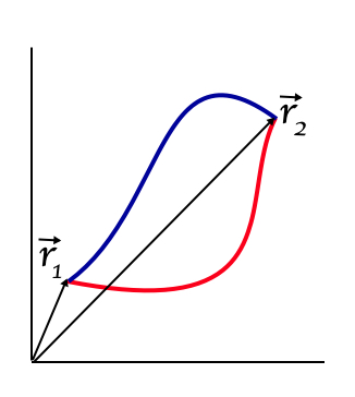
Fig. 5.1 Two different paths.

However, there is a certain class of forces for which the path does not matter, only the start and end point do. These forces are called conservative forces. As a consequence, the work done by a conservative force over a closed path, i.e start and end are the same, is always zero. No matter which closed path is taken.

Conservative Force

\( \text{conservative force } \Leftrightarrow \oint \vec{F} \cdot d\vec{r} = 0 \text{ for }\textbf{ALL}\text{ closed paths} \)

5.2. Stokes’ Theorem

It was George Stokes who proved an important theorem, that we will use to turn the concept of conservative forces into a new and important concept.

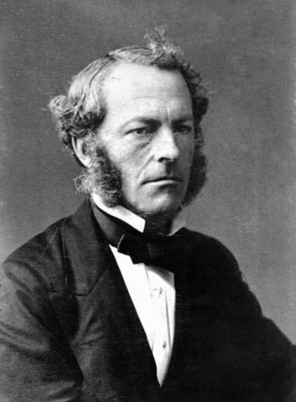
Fig. 5.2 Sir George Stokes (1819-1903). From Wikimedia Commons, public domain.

His theorem reads as:

\[ \oint \vec{F} \cdot d\vec{r} = \iint \vec{\nabla} \times \vec{F} \cdot d\vec{\sigma} \]

In words: the integral of the force over a closed path equals the surface integral of the curl of that force. The surface being ‘cut out’ by the close path. The term \(\vec{\nabla} \times \vec{F}\) is called the curl of \(F\): it is a vector. The meaning of it and some words on the theorem are given below.

Intermezzo: intuitive proof of Stokes’ Theorem

Consider a closed curve in the \(xy\)-plane. We would like to calculate the work done when going around this curve. In other words: what is \(\oint \vec{F} \cdot d\vec{r}\) if we move along this curve?

We can visualize what we need to do: we cut the curve in small part; compute \(\vec{F} \cdot d\vec{r}\) for each part (i.e. the red, green, blue, etc. in Fig. 5.3 and sum these to get the total along the curve. If we make the parts infinitesimally small, we go from a (Riemann) sum to an integral.

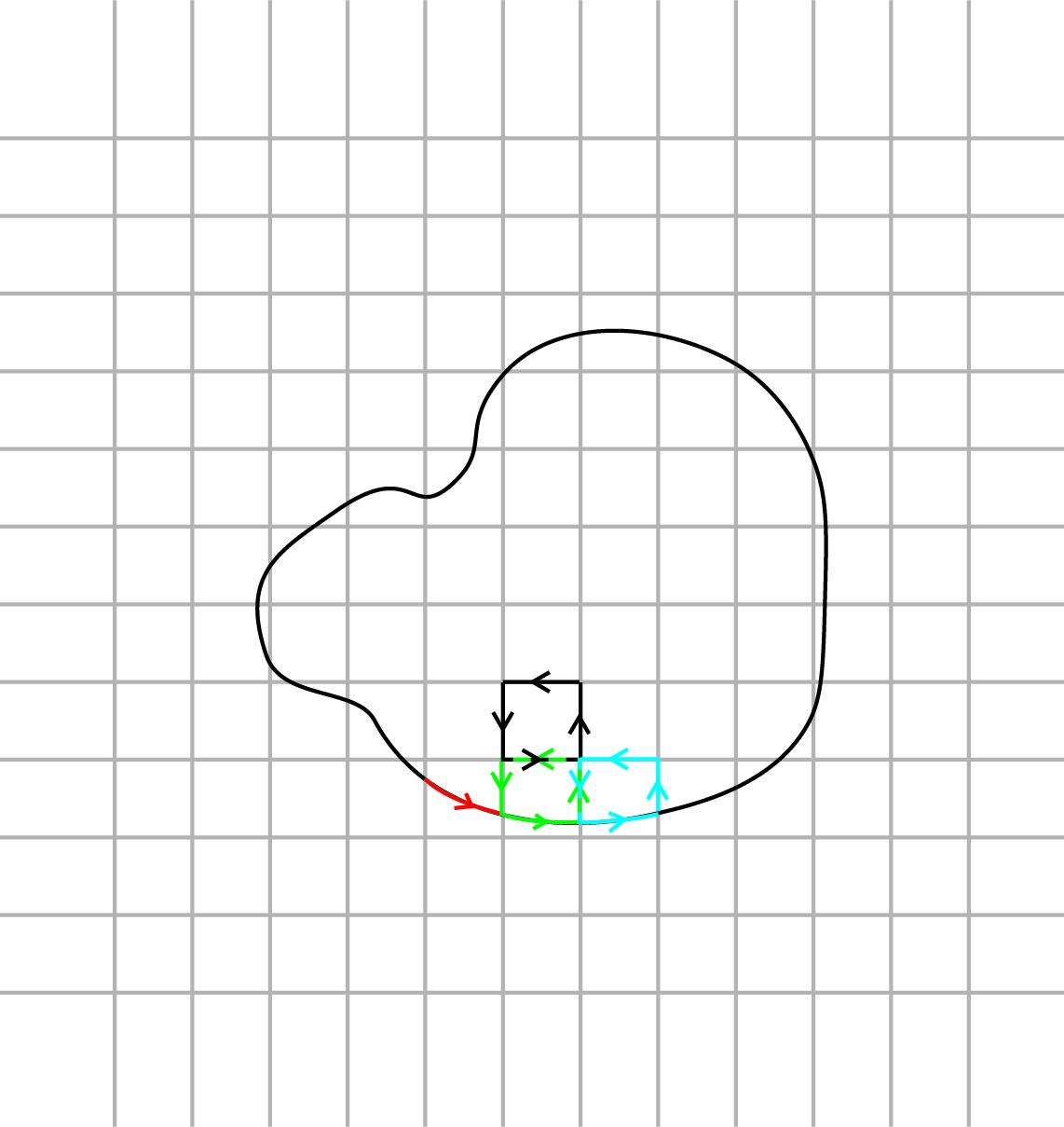
Fig. 5.3 Closed path on a grid.

We are going to compute much more: take a look at Fig. 5.3. We have put a grid in the \(xy\)-plane over a closed curve \(\Gamma\). Hence, the interior of our curve is full of squares. We are not only computing the parts along the curve, but also along the sides of all curves. This will sound like way too much work, but we will see that it actually is a very good idea.

See Fig. 5.3: we calculate \(\oint \vec{F} \cdot d\vec{r}\) counter clockwise for the green square. Now, we have at least the green part of our \(\oint \vec{F} \cdot d\vec{r}\) done in the right direction. But now we also compute \(\int \vec{F} \cdot d\vec{r}\) along the right side of the green square. We do that from bottom to top as we go counter clockwise along the green square. Let’s call that \(\int_g \vec{F} \cdot d\vec{r}\).

Then we move to the blue square and repeat in counter clockwise direction our calculation. But this means that we compute along the left side of the blue square from top to bottom. We will call this \(\int_b \vec{F} \cdot d\vec{r}\).

Note that we will add all contributions. Thus, we get \(\int_g \vec{F} \cdot d\vec{r} + \int_b \vec{F} \cdot d\vec{r}\). But these two cancel each other as they are exactly the same but done in opposite directions. Thus if we use that \(\int_1^2 f dx = - \int_2^1 f dx\) for any integration, it becomes obvious that \(\int_g \vec{F} \cdot d\vec{r} + \int_b \vec{F} \cdot d\vec{r} = 0\).

Note that this will happen for all side of the squares that are in the interior of our curve. Thus, the integral over all squares is exactly the integral along the curve \(\Gamma\).

It seems, we do a lot of work for nothing. But there is another way of looking at the path-integrals along the squares. If we make the square small enough, the calculation along one square can be approximated:

\[\begin{split} \begin{split} \oint_{square} \vec{F} \cdot d\vec{r} &\approx F_x(x,y) dx + F_y(x+dx,y) dy - F_x (x,y+dy) dx - F_y(x,y) dy \\ & \approx \frac{F_x(x,y) - F_x (x,y+dy)}{dy} dxdy + \frac{F_y(x+dx,y) - F_y(x,y) }{dx} dxdy \\ & \approx \left ( \frac{\partial F_y}{\partial x} - \frac{\partial F_x}{\partial y} \right ) dx dy \end{split} \end{split}\]

The results get more accurate the smaller we make the square.

If we now sum up all squares and make these squares infinitesimally small, the sum becomes an integral, but now an integral over the surface enclosed by the curve:

\[ \oint_{\Gamma} \vec{F} \cdot d\vec{r} = \iint \left ( \frac{\partial F_y}{\partial x} - \frac{\partial F_x}{\partial y} \right ) dx dy \]

The right hand side of the above equation is an surface integral of the ‘vector’ \(\frac{\partial F_y}{\partial x} - \frac{\partial F_x}{\partial y}\). Obviously, we did not provide a rigorous proof, but only an intuitive one. For a mathematical proof, see your calculus classes.

Moreover, we only worked in the \(xy\)-plane. If we would extend our reasoning to a closed curve in 3 dimensions, we would get Stokes theorem, which reads as:

\[ \oint_{\Gamma} \vec{F} \cdot d\vec{r} = \iint \vec{\nabla} \times \vec{F} \cdot d\vec{\sigma} \]

Here, \(d\vec{\sigma}\) is a small element out of the surface. Note that it is a vector: it has size and directions. The latter is perpendicular to the surface element itself. Furthermore, we have the vector \(\vec{\nabla} \times \vec{F}\). This is the cross-product of the nabla-operator and our vector field \(\vec{F}\). The nabla operator is a strange kind of vector. Its components are: partial differentiation. In a Cartesian coordinate system this can be written as:

\[ \vec{\nabla} \equiv \frac{\partial}{\partial x} \hat{x} + \frac{\partial}{\partial y} \hat{y} + \frac{\partial}{\partial z} \hat{z} \]

or if you prefer a column notation:

\[\begin{split} \vec{\nabla} \equiv \left ( \begin{matrix} \frac{\partial}{\partial x} \\ \frac{\partial}{\partial y} \\ \frac{\partial}{\partial z} \end{matrix} \right ) \end{split}\]

The curl of \(F\) can be found from e.g.

\[\begin{split} \vec{\nabla} \times \vec{F} = \begin{vmatrix} \hat{x} & \hat{y} & \hat{z} \\ \frac{\partial}{\partial x} & \frac{\partial}{\partial y} & \frac{\partial}{\partial z} \\ F_x & F_y & F_z \end{vmatrix} = \left ( \frac{\partial F_z}{\partial y} - \frac{\partial F_y}{\partial z} \right ) \hat{x} + \left ( \frac{\partial F_x}{\partial z} - \frac{\partial F_z}{\partial x} \right ) \hat{y} + \left ( \frac{\partial F_y}{\partial x} - \frac{\partial F_x}{\partial y} \right ) \hat{z} \end{split}\]

Note of warning: do be careful with the nabla-operator. It is not a standard vector. For instance, ordinary vectors have the property \(\vec{a} \cdot \vec{b} = \vec{b} \cdot \vec{a}\). This does not hold for the nabla-operator.

Second note of warning: the representation of the nabla-operator does change quite a bit when using other coordinate systems like cylindrical or spherical. For instance, in cylindrical coordinates it is not equal to \(\left ( \begin{matrix} \frac{\partial}{\partial r} \\ \frac{\partial}{\partial \phi} \\ \frac{\partial}{\partial z} \end{matrix} \right )\). This can be easily seen as both \(r, z\) have units length, i.e. meters, but \(\phi\) has no units.

Example 5.1

Suppose we need to calculate the integral of the vectorfield \(\vec{F}(x,y) = y \hat{x} - x \hat{y}\) over the closed curve formed by a square from \((0,0)\) to \((1,0)\), \((1,1)\), \((0,1)\) and back to \((0,0)\).

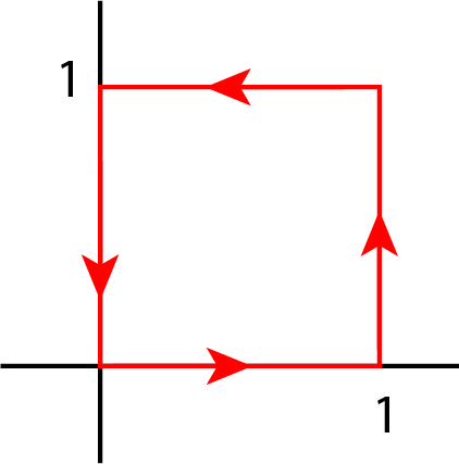
Fig. 5.4 Integrating along the unit square.

We go counter clockwise.

\[\begin{split} \begin{split} \oint \vec{F} \cdot d\vec{r} &= \int_{x=0}^1 F_x(x,y=0) dx + \int_{y=0}^1 F_y(x=1,y) dy + \\ & \;\; + \int_{x=1}^0 F_x(x,y=1) dx + \int_{y=1}^0 F_y(x=0,y) dy \\ &= \int_0^1 0 dx + \int_0^1 -1 dy + \int_1^0 1 dx + \int_1^0 -0 dx \\ &= 0 - [y]_0^1 + [x]_1^0 - 0 \\ &= -2 \end{split} \end{split}\]

Now we try this using Stokes’ Theorem:

\[ \oint \vec{F} \cdot d\vec{r} = \iint \vec{\nabla} \times \vec{F} \cdot d\vec{\sigma} \]

We first calculate \(\vec{\nabla} \times \vec{F}\):

\[\begin{split} \vec{\nabla} \times \vec{F} = \begin{vmatrix} \hat{x} & \hat{y} & \hat{z} \\ \frac{\partial}{\partial x} & \frac{\partial}{\partial y} & \frac{\partial}{\partial z} \\ F_x & F_y & F_z \end{vmatrix} = \begin{vmatrix} \hat{x} & \hat{y} & \hat{z} \\ \frac{\partial}{\partial x} & \frac{\partial}{\partial y} & \frac{\partial}{\partial z} \\ y & -x & 0 \end{vmatrix} = \left ( \frac{\partial (-x)}{\partial x} - \frac{\partial (y)}{\partial y} \right ) \hat{z} = -2 \hat{z} \end{split}\]

Thus, in this example \(\vec{\nabla} \times \vec{F}\) has only a \(z\)-component.

An elementary surface element of the square is: \(d\vec{\sigma} = dx dy \hat{z}\). This also has only a \(z\)-component. Note that it points in the positive \(z\)-direction. This is a consequence of the counter clockwise direction that we use to go along the square.

According to Stokes Theorem, we this find:

\[ \oint \vec{F} \cdot d\vec{r} = \iint \vec{\nabla} \times \vec{F} \cdot d\vec{\sigma} = \int_{x=0}^1 \int_{y=0}^1 (-2) dxdy = -2 \]

Indeed, we find the same outcome.

5.3. Conservative force and \(\vec{\nabla} \times \vec{F}\)

For a conservative force the integral over the closed path is zero for any closed path. Consequently, \( \vec{\nabla} \times \vec{F} = 0 \) everywhere. How do we know this? Suppose \( \vec{\nabla} \times \vec{F} \neq 0 \) at some point in space. Then, since we deal with continuous differentiable vector fields, in the close vicinity of this point, it must also be non-zero. Without loss of generality, we can assume that in that region \( \vec{\nabla} \times \vec{F} \cdot d\vec{\sigma}> 0 \). Next, we draw a closed curve around this point, in this region. We now calculate the \(\oint \vec{F} \cdot d\vec{r}\) along this curve. That is, we invoke Stokes Theorem. But we know that \( \vec{\nabla} \times \vec{F} \cdot d\vec{\sigma} > 0 \) on the surface formed by the closed curve. Consequently, the outcome of the surface integral is non-zero. But that is a contradiction as we started with a conservative force and thus the integral should have been zero.
The only way out, is that \( \vec{\nabla} \times \vec{F} = 0 \) everywhere.

Thus we have:

Conservative Force

\(\text{conservative force } \Leftrightarrow \vec{\nabla} \times \vec{F} = 0 \text{ everywhere} \)

5.4. Potential Energy

A direct consequence of the above is:

if \( \vec{\nabla} \times \vec{F} = 0 \) everywhere, a function \( V (\vec{r})) \) exists such that \( \vec{F} = -\vec{\nabla}V \)

\[\begin{split} \text{conservative force } \Leftrightarrow \vec{\nabla} \times \vec{F} = 0 \text{ everywhere } \\ \big\Updownarrow \\ \vec{F} = -\vec{\nabla}V \Leftrightarrow V(\vec{r}) = -\int_{ref} \vec{F} \cdot d\vec{r} \end{split}\]

where in the last integral, the lower limit is taken from some, self picked, reference point. The upper limit is the position \( \vec{r} \).

Potential Energy

if F is conservative a Potential Energy exists:

\( \vec{F} = -\vec{\nabla}V \Leftrightarrow V(\vec{r}) = -\int_{ref} \vec{F} \cdot d\vec{r} \)

This function V is called the potential energy or the potential for short. It has a direct connection to work and kinetic energy.

\[ E_{kin,2} - E_{kin,1} = W_{12} = \int_1^2 \vec{F} \cdot d\vec{r} = V(\vec{r}_2) - V(\vec{r}_1) \]

or rewritten:

\[ E_{kin,1} + V(\vec{r}_1) = E_{kin,2} + V(\vec{r}_2) \]

In words: for a conservative force, the sum of kinetic and potential energy stays constant.

Conservation of Energy

for a conservative force, the sum of kinetic and potential energy stays constant

\( E_{kin} + V(\vec{r}) = E_0 \)

5.4.1. Energy versus Newton’s Second Law

We, starting from Newton’s Laws, arrived at an energy formulation for physical problems.
Question: can we also go back? That is: suppose we would start with formulating the energy rule for a physical problem, can we then back out the equation of motion?
Answer: yes, we can!

It goes as follows. Take a system that can be completely described by its kinetic plus potential energy. Then: take the time-derivative and simplify, we will do it for a 1-dimensional case first.

\[\begin{split}\begin{split} &\frac{1}{2}mv^2 + V(x) = E_0 \Rightarrow \\ &\frac{d}{dt} \left [ \frac{1}{2}mv^2 + V(x) \right ] = \frac{dE_0}{dt} = 0 \Rightarrow \\ &mv\dot{v} + \frac{dV}{dx}\underbrace{\frac{dx}{dt}}_{=v} = 0 \Rightarrow \\ &v \left (m\dot{v} + \frac{dV}{dx} \right ) = 0 \end{split}\end{split}\]

The last equation must hold for all times and all circumstances. Thus, the term in brackets must be zero.

\[ m\dot{v} + \frac{dV}{dx} = 0 \Rightarrow m\ddot{x} = -\frac{dV}{dx} = F \]

And we have recovered Newton’s second law.

In 3 dimensions it is the same procedure. What is a bit more complicated, is using the chain rule. In the above 1-d case we used \(\frac{dV}{dt} = \frac{dV(x(t))}{dt} = \frac{dV}{dx}\frac{dx(t)}{dt}\). In 3-d this becomes:

\[\frac{dV}{dt} = \frac{dV(\vec{r}(t))}{dt} = \frac{dV}{d\vec{r}}\cdot \frac{d\vec{r}(t)}{dt} = \vec{\nabla} V \cdot \vec{v} \]

Thus, if we repeat the derivation, we find:

\[\begin{split}\begin{split} &\frac{1}{2}mv^2 + V(\vec{r}) = E_0 \Rightarrow \\ &\frac{d}{dt} \left [ \frac{1}{2}mv^2 + V(\vec{r}) \right ] = 0 \Rightarrow \\ &m\vec{v} \cdot \dot{\vec{v}} + \vec{\nabla} V \cdot \vec{v} = 0 \Rightarrow \\ &v \left (m\vec{a} + \vec{\nabla} V \right ) = 0 \Rightarrow \\ &m\vec{a} = -\vec{\nabla} V = \vec{F} \end{split}\end{split}\]

And we have recovered the 3-dimensional form of Newton’s second Law. This is a great result. It allows us to pick what we like: formulate a problem in terms of forces and momentum, i.e. Newton’s second law, or reason from energy considerations. It doesn’t matter: they are equivalent. It is a matter of taste, a matter of what do you see first, understand best, find easiest to start with. Up to you!

5.5. Stable/Unstable Equilibrium

A particle (or system) is in equilibrium when the sum of forces acting on it is zero. Then, it will keep the same velocity, and we can easily find an inertial system in which the particle is at rest, at an equilibrium position.
The equilibrium position (or more general state) can also be found directly from the potential energy.

Potential energy and (conservative) forces are coupled via:

\[ \vec{F} = - \vec{\nabla}V \]

The equilibrium positions \(\left ( \sum_i \vec{F}_i = 0 \right )\) can be found by finding the extremes of the potential energy:

\[ \text{equilibrium position } \Leftrightarrow \vec{\nabla}V = 0 \]

Once we find the equilibrium points, we can also quickly address their nature: is it a stable or unstable solution? That follows directly from inspecting the characteristics of the potential energy around the equilibrium points.

For a stable equilibrium, we require that a small push or a slight displacement will result in a force pushing back such that the equilibrium position is restored (apart from the inertia of the object that might cause an overshoot or oscillation).

However, an unstable equilibrium is one for which the slightest push or displacement will result in motion away from the equilibrium position.

The second derivative of the potential can be investigated to find the type of extremum. For 1D functions that is easy, for scalar valued functions of more variables that is a bit more complicated. Here we only look at the 1D case \(V(x): \mathbb{R} \rightarrow \mathbb{R}\)

\[\begin{split} \text{equilibrium: } \vec{\nabla}V = 0 \begin{cases} \text{stable: } & \frac{d^2V}{dx^2} > 0 \\ \text{unstable: } & \frac{d^2V}{dx^2} < 0 \end{cases} \end{split}\]

Luckily, the definition of potential energy is such that these rules are easy to visualize in 1D and remember, see Fig. 5.5.

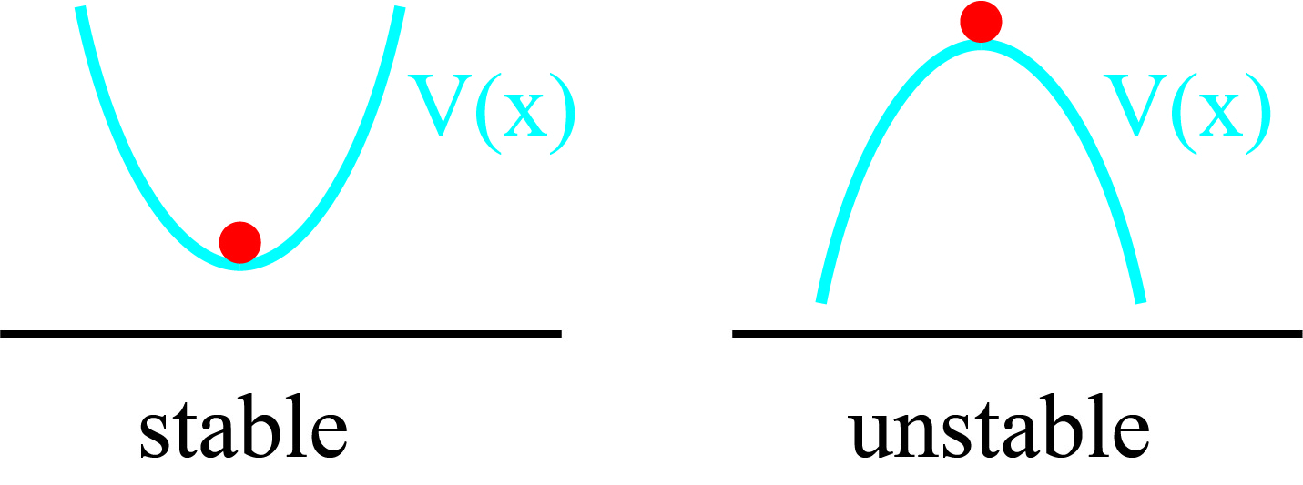
Fig. 5.5 Stable and unstable position of a particle in a potential.

A valley is stable; a hill top is unstable.
NB: Now the choice of the minus sign in the definition of the potential is clear . Otherwise a hill would be stable, but that does not feel natural at all.

It is also easy to visualize what will happen if we distort that particle from the equilibrium state:

• The valley, i.e., the stable system, will make the particle move back to the lowest point. Due to inertia, it will not stop but will continue to move. As the lowest position is one of zero force, the particle will 'climb' toward the other end of the valley and start an oscillatory motion.
• The top, i.e., the unstable point, will make the particle move away from the stable point. The force acting on the particle is now pushing it outwards, down the slope of the hill.

5.5.1. Taylor Series Expansion of the Potential

The Taylor expansion or Taylor series is a mathematical approximation of a function in the vicinity of a specific point. It uses an infinite series of polynomial terms with coefficients given by value of the derivative of the function at that specific point: the more terms you use, the better the approximation. If you use all terms, then it is exact. Mathematically, it reads for a 1D scalar function \(f: \mathbb{R} \rightarrow \mathbb{R}\):

\[ f(x) \approx f(x_0) + \frac{1}{1!} f'(x_0) (x-x_0 ) + \frac{1}{2!} f''(x_0) (x-x_0)^2 + \frac{1}{3!} f'''(x_0) (x-x_0)^3 + ... \]

For our purpose here, it suffices to stop after the second derivative term:

\[ f(x) \approx f(x_0) + f'(x_0) (x-x_0 ) + \frac{1}{2} f''(x_0) (x-x_0)^2 + \mathcal{O}(x^3) \]

A way of understanding why the Taylor series actually works is the following.
Imagine you have to explain to someone how a function looks around some point \(x_0\), but you are not allowed to draw it. One way of passing on information about \(f(x)\) is to start by giving the value of \(f(x)\) at the point \(x_0\):

\[ f(x) \approx f(x_0) \]

Next, you give how the tangent at \(x_0\) is; you pass on the first derivative at \(x_0\). The other person can now see a bit better how the function changes when moving away from \(x_0\):

\[ f(x) \approx f(x_0) + f'(x_0) (x-x_0 ) \]

Then, you tell that the function is not a straight line but curved, and you give the second derivative. So now the other one can see how it deviates from a straight line:

\[ f(x) \approx f(x_0) + \frac{1}{1!} f'(x_0) (x-x_0 ) + \frac{1}{2!} f''(x_0) (x-x_0)^2 \]

Note that the prefactor is placed back. But the function is not necessarily a parabola; it will start deviating more and more as we move away from \(x_0\). Hence we need to correct that by invoking the third derivative that tells us how fast this deviation is. And this process can continue on and on.

Important to note: if we stay close enough to \(x_0\) the terms with the lowest order terms will always prevail as higher powers of \((x-x_0)\) tend to zero faster than a lower powers (for instance: \(0.5^4 << 0.5^2\)).

Here is a youtube movie that explains the 1D Taylor series nicely (for physicists).

For scalar valued functions as our potentials \(V(\vec{r}): \mathbb{R}^3 \rightarrow \mathbb{R}\) the extension of the Taylor series is not too difficult. If we expand the function around a point

\[\begin{split}\begin{split} V(\vec{r}) &\approx V(\vec{r}_0) + \vec{\nabla}V(\vec{r}_0) \cdot (\vec{r}-\vec{r}_0 ) \\ &+ \frac{1}{2} (\vec{r}-\vec{r}_0 ) \cdot (\partial^2 V)(\vec{r}_0) \cdot (\vec{r}-\vec{r}_0 ) + \mathcal{O}(r^3) \end{split}\end{split}\]

The second derivative of the potential indicated by \(\partial^2 V\) is the Hessian matrix.

Conceptually the extrema of the function are again the hills and valleys. The classification of the extrema has next to hills and valleys also saddle points etc. In this course we will not bother about these more dimensional cases, but only stick to simple ones.

5.5.2. Examples & Exercises

Example 5.2

Is gravity \( \vec{F}_g = m\vec{g} \) a conservative force? If yes, what is the corresponding potential energy?

To find the answer we can do two things:

   a. Show \( \vec{\nabla} \times m\vec{g} = 0 \)
   b. Find a \(V\) that satisfies \( -m\vec{g} = -\vec{\nabla} V \)

Solution Example 5.2

   a. \( \vec{\nabla} \times m\vec{g} = 0 \)? How to compute it? For Cartesian coordinates there is an easy to remember rule:

\[\begin{split} \vec{\nabla} \times \vec{F} = \begin{vmatrix}\hat{x}&\hat{y}&\hat{z}\\\frac{\partial}{\partial x}&\frac{\partial}{\partial y}&\frac{\partial}{\partial z}\\F_x&F_y&F_z\end{vmatrix} \end{split}\]

If we chose our coordinates such that \( \vec{g} = -g \hat{z} \) we get: $\(\vec{\nabla} \times \vec{F}_g = \begin{vmatrix}\hat{x}&\hat{y}&\hat{z}\\\frac{\partial}{\partial x}&\frac{\partial}{\partial y}&\frac{\partial}{\partial z}\\0&0& -mg\end{vmatrix} = 0\)\( Thus \) \vec{F}_g $ is conservative.

   b. Secondly: does \( -m\vec{g} = -\vec{\nabla} V \) have a solution for V? Let’s try, using the same coordinates as above. $\(\begin{split} -\vec{\nabla}V &= - m\vec{g} \Rightarrow \\ \frac{\partial V}{\partial x} &= 0 \rightarrow V(x,y,z) = f(y,z) \\ \frac{\partial V}{\partial y} &= 0 \rightarrow V(x,y,z) = g(x,z) \\ \frac{\partial V}{\partial z} &= mg \rightarrow V(x,y,z) = mgz + h(x,y) \end{split} \)$

f,g,h are unknow functions. But all we need to do, is find one \(V\) that satisfies \( -m\vec{g} = -\vec{\nabla} V \).

So, if we take \( V(x,y,z) = mgz \) we have shown, that gravity in this form is conservative and that we can take \( V(x,y,z) = mgz \) for its corresponding potential energy.

By the way: from the first part (curl F = 0), we know that the force is conservative and we know that we could try to find V from

\[\begin{split} \begin{split} V(x,y,z) &= -\int_{ref} m\vec{g} \cdot d\vec{r} = \int_{ref} mg \hat{z} \cdot d\vec{r} \\ &= \int_{ref} mg dz = mgz + const \end{split} \end{split}\]

Exercise 5.1

A simple model for the frictional force experienced by a body sliding over a horizontal, smooth surface is \( F_f = -\mu F_g \) with \( F_g \) the gravitational force on the object.The friction force is opposite the direction of motion of the object.

• Show that this frictional force is not conservative (and, consequently, a potential energy associated does not exist!).

Hint: think of two different trajectories to go from point 1 to point 2 and show that the amount of work along these trajectories is not the same.

Exercise 5.2

A force is given by: \( \vec{F} = x\hat{x} + y\hat{y} + z\hat{z} \)

1. Show that this force is conservative.
2. Find the corresponding potential energy.

A second force is given by: \( \vec{F} = y\hat{x} + x\hat{y} + z\hat{z} \)

1. Show that this force is also conservative.
2. Find the corresponding potential energy.

Exercise 5.3

Another force is given by: \( \vec{F} = y\hat{x} - x\hat{y} \)

1. Show that this frictional force is not conservative.
2. Compute the work done when moving an object over the unit circle in the xy-plane in an anti-clockwise direction.
   Hint: use Stokes theorem.
3. Discuss the meaning of your answer: is it positive or negative? And what does that mean in terms of physics?

Exercise 5.4

Given a potential energy \( E_{pot} = xy\).
   a. Find the corresponding force (field).
   b. Make a plot of \( \vec{F} \) as a function of (x,y,z).
   c. Describe the force and comment on what the potential itself already reveals about the force.

Exercise 5.5

Given a force field \( \vec{F} = -xy \hat{x} + xy \hat{y} \). A particle moves from \( (x,y) = (0,0) \) over the x-axis to \( (x,y) = (1,0) \) and then parallel to the y-axis to \( (x,y) = (1,1) \). In a second motion, the same particle goes from \( (x,y) = (0,0) \) over the y-axis to \( (x,y) = (0,1) \) and then parallel to the x-axis to end also in \( (x,y) = (1,1) \).

1. Show that not necessarily the work done over the two paths is equal.
2. Compute the amount of work done over each of the paths.

Exercise 5.6

A particle of mass m is initially at position \( x=0\). It has zero velocity.
On the particle a force is acting. The force can be described by \( F = F_0 \sin \frac{x}{L} \) with \( F_0 \) and \( L \) positive constants.

   a. Show that this force is conservative and find the corresponding potential. Take as reference point for the potential energy \( x = \frac{\pi}{2} L \).
   b. The particle gets a tiny push, such that it starts moving in the positive x-direction. Its initial velocity is so small that, for all practical calculations, it can be set to zero. Under the influence of the force, the particle will move. Why did the particle get its tiny push?
   c. Find the maximum velocity that the particle can get. At which location(s) will this take place?.

Note: this is a 1-dimensional problem.

5.5.3. Answers

Solution to Exercise 5.1

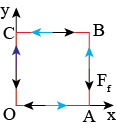
a) see figure: make two different paths along the red square in the xy-plane:
path 1: O=(0,0) → C=(0,1)
path 2: O → A=(1,0) → B=(1,1) → C
The blue arrows indicate the direction of traveling; the black arrows the friction force on each piece of the paths.

b) compute work done moving over path 1:

\[W_{OC} = \int_0^1 -\mu mgdy = −\mu mg \]

Compute work done moving over path 2:

\[W_{OABC} = ∫_0^1 -\mu mg dx + \int_0^1 -\mu mgdy + \int_1^0 \mu mgdx = -3\mu mg\]

Clearly the work done for the two paths are not equal. Thus, this force in not conservative.

Solution to Exercise 5.2

No sketch needed: this is a purely mathematical exercise.
1)a)

\[\begin{split} \vec{\nabla} \times \vec{F} = \begin{vmatrix}\hat{x}&\hat{y}&\hat{z}\\\frac{\partial}{\partial x}&\frac{\partial}{\partial y}&\frac{\partial}{\partial z}\\F_x&F_y&F_z\end{vmatrix} = \begin{vmatrix}\hat{x}&\hat{y}&\hat{z}\\\frac{\partial}{\partial x}&\frac{\partial}{\partial y}&\frac{\partial}{\partial z}\\x&y&z\end{vmatrix} = 0 \end{split}\]

thus F is conservative and a potential exists.

b)

\[ \vec{F} = -\vec{\nabla} V \Rightarrow\]

\[\begin{split}\begin{split} \frac{\partial V}{\partial x} &= -F_x = -x \rightarrow V(x,y,z) -\frac{1}{2}x^2 + f(y,z) \\ \frac{\partial V}{\partial y} &= -F_y = -y \rightarrow V(x,y,z) -\frac{1}{2}y^2 + g(x,z) \\ \frac{\partial V}{\partial z} &= -F_z = -z \rightarrow V(x,y,z) -\frac{1}{2}z^2 + h(x,y) \end{split}\end{split}\]

Thus, we can take:

\[ V(x,y,z) = -\frac{1}{2} x^2 - \frac{1}{2}y^2 -\frac{1}{2}z^2 +C\]

With \(C\) any constant we like.

2)a)

\[\begin{split} \vec{\nabla} \times \vec{F} = \begin{vmatrix}\hat{x}&\hat{y}&\hat{z}\\\frac{\partial}{\partial x}&\frac{\partial}{\partial y}&\frac{\partial}{\partial z}\\F_x&F_y&F_z\end{vmatrix} = \begin{vmatrix}\hat{x}&\hat{y}&\hat{z}\\\frac{\partial}{\partial x}&\frac{\partial}{\partial y}&\frac{\partial}{\partial z}\\y&x&z\end{vmatrix} = 0\hat{x} + 0\hat{y} + \left ( \frac{\partial}{\partial x} x - \frac{\partial}{\partial y} y \right )\hat{z} = 0 \end{split}\]

thus F is conservative and a potential exists.

b) $\( \vec{F} = -\vec{\nabla} V \Rightarrow\)$

\[\begin{split}\begin{split} \frac{\partial V}{\partial x} &= -F_x = -y \rightarrow V(x,y,z) -xy + f(y,z) \\ \frac{\partial V}{\partial y} &= -F_y = -x \rightarrow V(x,y,z) -xy + g(x,z) \\ \frac{\partial V}{\partial z} &= -F_z = -z \rightarrow V(x,y,z) -\frac{1}{2}z^2 + h(x,y) \end{split}\end{split}\]

Thus, we can take:

\[ V(x,y,z) = -xy -\frac{1}{2}z^2 +C\]

With \(C\) any constant we like.

Solution to Exercise 5.3

a)

\[\begin{split} \vec{\nabla} \times \vec{F} = \begin{vmatrix}\hat{x}&\hat{y}&\hat{z}\\\frac{\partial}{\partial x}&\frac{\partial}{\partial y}&\frac{\partial}{\partial z}\\F_x&F_y&F_z\end{vmatrix} = \begin{vmatrix}\hat{x}&\hat{y}&\hat{z}\\\frac{\partial}{\partial x}&\frac{\partial}{\partial y}&\frac{\partial}{\partial z}\\y&-x&0\end{vmatrix} = 0\hat{x} + 0\hat{y} + \left ( \frac{\partial}{\partial x} (-x) - \frac{\partial}{\partial y} y \right )\hat{z} = -2\hat{z} \end{split}\]

thus F is not conservative.

b) Stokes’ Theorem

\[\oint \vec{F} \cdot d\vec{r} = \iint\vec{\nabla} \times \vec{F} \cdot d\vec{\sigma}\]

We take the unit circle in the xy-plane as our closed curve. The surface element is \( d\vec{\sigma} = +dxdy \hat{z} \) (note the +sign for de surface element: we ‘walk’ counter-clockwise over the unit circle). Furthermore, we already computed \(\vec{\nabla} \times \vec{F} = -2\hat{z}\).

Thus: $\(W = \oint \vec{F} \cdot d\vec{r} = \iint\vec{\nabla} \times \vec{F} \cdot d\vec{\sigma} = -2\underbrace {\hat{z}\cdot\hat{z}}_{=1} \underbrace{\iint_{unit circle} dxdy}_{\pi 1^2} = -2\pi\)$

c) Obviously, the work done is negative. This means that the kinetic energy of the object that is moved around is decreasing. The force is thus acting against the motion. You can easily check this for yourself by drawing at a few positions on the unit circle the direction of the force.

Solution to Exercise 5.4

a) Given \( E_{pot} = V(x,y) = xy \rightarrow \vec{F} = - \vec{\nabla}V = -\frac{\partial V}{\partial x} \hat{x} -\frac{\partial V}{\partial y} \hat{y} -\frac{\partial V}{\partial z} \hat{z} = -x\hat{x} - y\hat{y}\).

b)

c) The force is attracting towards the origin. The further away from the origin the stronger the force.
It can be directly seen from the potential that the force points ‘inwards’: the further away from the origin the higher the potential energy. A particle will have the tendency to move down the potential energy, i.e. to lower values.
Moreover, the potential is an odd function in both \(x\) and \(y\), reflecting the symmetry of the force around the \(x\)- and \(y\)-axis.

Solution to Exercise 5.5

a) Given \( \vec{F} = -xy\hat{x} + xy\hat{y}\).
Conservative?

\[\begin{split} \vec{\nabla} \times \vec{F} = \begin{vmatrix}\hat{x}&\hat{y}&\hat{z}\\\frac{\partial}{\partial x}&\frac{\partial}{\partial y}&\frac{\partial}{\partial z}\\F_x&F_y&F_z\end{vmatrix} = \begin{vmatrix}\hat{x}&\hat{y}&\hat{z}\\\frac{\partial}{\partial x}&\frac{\partial}{\partial y}&\frac{\partial}{\partial z}\\-xy&xy&0\end{vmatrix} = \left ( \frac{\partial}{\partial x} (xy) - \frac{\partial}{\partial y} (-xy) \right )\hat{z} = (x+y)\hat{z} \end{split}\]

This is not zero everywhere. Hence this is a non-conservative force. Consequently, the work done over a path does not only depend on the start and end point but -in general- also on the path itself.

b)

Path \(OAP\):

\[W_{OAP} = \int_{x=0,y=0}^{x=1,y=0} F_x dx + \int_{x=1,y=0}^{x=1,y=1} F_y dy = 0\int_0^1 (-x)dx + 1 \int_0^1 ydy = \frac{1}{2}\]

Path \(OBP\):

\[W_{OBP} = \int_{x=0,y=0}^{x=0,y=1} F_y dy + \int_{x=0,y=1}^{x=1,y=1} F_x dx = 0\int_0^1 ydy + 1 \int_0^1 (-x)dx) = -\frac{1}{2}\]

Indeed, the amount of work turns out to be path dependent. We could expect this based on (a). However, if a force is not conservative it does not mean that the work done when going from point 1 to point 2 will always be different for different paths. It may very well be that the amount of work along some paths (or even many) will be the same.
It does mean that there are paths that give different outcomes. Or rephased: if a force is not-conservative then “not for every closed path is the amount of work done zero”.

Solution to Exercise 5.6

a) Given \(F=F_0 \sin \frac{x}{L}\)
If conservative, a potential does exist. So, if we can find the potential, then we know F is conservative:

\[V=-\int_{\frac{\pi}{2}L}^x F(x')dx' = F_0 L \left [ \cos \frac{x'}{L}\right ]_{\frac{\pi}{2}L}^x = F_0 L \cos \frac{x}{L}\]

So, we found a potential and thus F is conservative.

b) The particle is initially at \(x= 0\). At this point the force \(F = 0\). Consequently, the particle will not move. However, the slightest push will have it move away from the point \(x=0\). As soon as the particle is out of \(x=0\) it does experience a non-zero force and will move.

c) The total energy of the particle is constant. This means that

\[ \frac{1}{2}mv^2 + F_0L \cos \frac{x}{L} = E_0\]

Initially, \(v=0\) (that is so small that for all practical calculations the initial kinetic energy can be taken as zero). Thus

\[E_0 = F_0 L \cos 0 = F_0 L\]

and

\[ v = \sqrt{\frac{2}{m} \left ( F_0 L - F_0 L \cos \frac{x}{L} \right )}\]

This has a maximum when the cos-term has a minimum. This happens at

\[ x = (\pi \pm 2k\pi)L\]

At these positions

\[v_{max} = 2\sqrt{\frac{F_0L}{m}}\]