11. Two Body Problem: Kepler revisited

Newton must have realized that his analysis of the Kepler laws was not 100% correct. After all, the sun is not fixed in space and even though its mass is much larger than any of the planets revolving it, it will have to move under the influence of the gravitational force by the planets. Take for example, the sun and earth as our system. By the account of Newton’s third law, the Earth exerts also a force on the Sun. Therefore, the Sun has to move as well; thus, we must revisit the Earth-Sun analysis and incorporate that the Sun isn’t fixed in space.

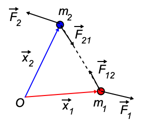
Fig. 11.1 Two-particle system, with an action/reaction pair of forces.

The two-body problem is stated hereby as:

Particle \(m_1\) feels an external force \(\vec{F}_1\) and an interaction force from particle two, \(\vec{F}_{21}\). Similarly for particle \(m_2\).

Consider the situation in the figure:

\[ m_1 \ddot{\vec{x}}_1 = \vec{F}_1 + \vec{F}_{21} \]

\[ m_2 \ddot{\vec{x}}_2 = \vec{F}_2 + \vec{F}_{12} \]

Add the two equations and use N3: \(\vec{F}_{12} = - \vec{F}_{21}\):

\[ m_1 \ddot{\vec{x}}_1 + m_2 \ddot{\vec{x}}_2 = \vec{F}_1 + \vec{F}_{2} \Leftrightarrow \]

\[ \dot{\vec{P}} = \vec{F}_{1} + \vec{F}_2 \]

with \(\vec{P} \equiv \vec{p}_1 + \vec{p}_2\). In words, it is as if a particle with (total) momentum \(\vec{P}\) responds to the external forces but does not react to internal forces (the mutual interaction).

11.1. Center of Mass

It is now logical to assign the total mass \(M=m_1+m_2\) to this fictitious particle. It has momentum \(\vec{p}_1+\vec{p}_2\) which we can also couple to its mass \(M\) and assign a velocity \(\vec{V}\) to it such that \(\vec{P}=M\vec{V}\). Furthermore, if this fictitious mass has velocity \(\vec{V}\), we can also assign a position to it. Afterall, \(\vec{V} = \frac{d\vec{R}}{dt}\), which gives us the recipe for the position \(\vec{R}\).

Its velocity \(\vec{V}\) and position \(\vec{R}\) then follow as:

\[\begin{split} \begin{split} \vec{V} &= \frac{m_1 \vec{v}_1 + m_2 \vec{v}_2 }{m_1 + m_2} \\ &= \frac{m_1 \frac{d\vec{x}_1}{dt} + m_2 \frac{d\vec{x}_2}{dt} }{m_1 + m_2}\\ \\ \Rightarrow \vec{R} &= \frac{m_1 \vec{x}_1 + m_2 \vec{x}_2}{m_1 + m_2} +\vec{C} \end{split} \end{split}\]

In the last equation, we have an integration constant in the form of a vector, \(\vec{C}\). We are free to choose it as we want: its precise value does not affect the velocity \(\vec{V}\) nor the momentum \(\vec{P}\) of our fictitious particle.

It makes sense, to choose: \(\vec{C} = 0\) and thus define as position of the particle:

\[ \vec{R} = \frac{m_1 \vec{x}_1 + m_2 \vec{x}_2}{m_1 + m_2} \]

Why?

We have a few arguments:

1. if the particles are actually each half of a real particle, we obviously require that \(\vec{R}\) is the position of the real particle.

2. If the particles are separate by a small distance, we would like to have the fictitious particle somewhere in between the two. Moreover, if the two particles are identical, it makes sense to have the fictitious particle right in between them: the system is symmetric.

Where, in general, is the position \(\vec{R}\)?
That can be easily seen from the figure below.

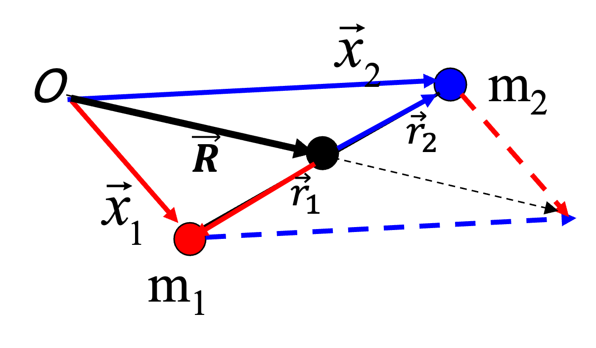
Fig. 11.2 Center of Mass and relative coordinates.

We rewrite the definition of \(\vec{R}\):

\[ \vec{R} \equiv \frac{m_1 \vec{x}_1 + m_2 \vec{x}_2}{m_1 + m_2} = \vec{x}_1 + \frac{m_2}{m_1 + m_2} \left ( \vec{x}_2 - \vec{x}_1\right )\]

Thus, the last part of the above equation tells us: first go to \(m_1\) and then, ‘walk’ a fraction \(\frac{m_2}{m_1 + m_2} \) of the line connecting \(m_1\) and \(m_2\). If you have done that, you are at position \(\vec{R}\).
Note: if \(m_1 = m_2\) this recipe indeed brings us right between the two particles.
Further note: the position of \(M\) is always on the line from \(m_1\) to \(m_2\). If \(m_1\) is much larger than \(m_2\), it will be located close to \(m_1\) and vice versa.

We call this position the center of mass, or CM for short. Reason: if we look at the response of our two particle system to the forces, it is as if there is a particle \(M\) at position \(\vec{R}\) that has all the momentum of the system.

It turns out to be convenient to define relative coordinates with respect to the center of mass position (see also the figure above):

\[ \vec{r}_1 \equiv \vec{x}_1 - \vec{R} \text{ and } \vec{r}_2 \equiv \vec{x}_2 - \vec{R} \]

Via the external forces, we can ‘follow’ the motion of the center of mass position, i.e. \(\vec{R}\). From the CM as new origin, we can find the position of the two particles.

A helpful rule is found from:

\[\begin{split} \begin{array}{l} m_1 \vec{r}_1 + m_2 \vec{r}_2 = \\ =m_1 \left ( \vec{x}_1 - \vec{R} \right ) + m_2 \left ( \vec{x}_2 - \vec{R} \right ) \\ =m_1 \vec{x}_1 + m_2 \vec{x}_2 - (m_1 + m_2 ) \vec{R} = 0 \end{array} \end{split}\]

\[ \Rightarrow m_1 \vec{r}_1 + m_2 \vec{r}_2 = 0 \]

This has an important consequence: if we know \(\vec{r}_1\), we know \(\vec{r}_2\), and vice versa. Note: the directions of \(\vec{r}_1\) and \(\vec{r}_2\) are always opposed and the center of mass \(\vec{R}\) is located somewhere on the connecting line between \(m_1\) and \(m_2\).

Note: in the case of no external forces \(\vec{F}_1=\vec{F}_2=0\) and only internal forces \(\vec{F}_{12} \neq 0\) the CM moves according to N1 with constant velocity \((\dot{\vec{P}}=0)\).

11.2. Energy

In terms of relative coordinates, we can write the kinetic energy as a part associated with the CM and a part that describes the kinetic energy with respect to the CM, i.e., ‘an internal kinetic energy.’

\[\begin{split} \begin{array}{rcl} E_{kin} &\equiv &\frac{1}{2} m_1 v_1^2 + \frac{1}{2} m_2 v_2^2 \\ &= &\frac{1}{2} m_1 \left ( \dot{\vec{r}}_1 + \dot{\vec{R}} \right )^2 + \frac{1}{2} m_2 \left ( \dot{\vec{r}}_2 + \dot{\vec{R}} \right )^2 \\ &= &\frac{1}{2} M \dot{\vec{R}}^2 + \frac{1}{2} m_1 \dot{\vec{r}}_1^2 + \frac{1}{2} m_2 \dot{\vec{r}}_2^2 \end{array} \end{split}\]

For the potential energy, we may write:

\[ V = \sum V_i + \frac{1}{2} \sum_{i \neq j} \left ( V_{ij} + V_{ji} \right ) \]

With \(V_i\) the potential related to the external force on particle \(i\) and \(V_{ij}\) the potential related to the mutual interaction force from particle \(i\) exerted on particle \(j\) (assuming that all forces are conservative).

11.3. Angular Momentum

The total angular momentum is, like the total momentum, defined as the sum of the angular momentum of the two particles:

\[ \vec{L} = \vec{l}_1 + \vec{l}_2 = \vec{x}_1 \times \vec{p}_1 + \vec{x}_2 \times \vec{p}_2 \]

We can write this in the new coordinates:

\[ \vec{L} = \vec{R} \times \vec{P} + \vec{r}_1 \times \vec{p}_1 + \vec{r}_2 \times \vec{p}_2 = \vec{L}_{cm} + \vec{L}' \]

We find: the total angular momentum can be seen as the contribution of the CM and the sum of the angular momentum of the individual particles as seen from the CM.

11.4. Reduced Mass

Suppose that there are no external forces. Then the equation of motion for both particles reads as:

\[\begin{split} \begin{array}{rcl} m_1 \ddot{\vec{x}_1} &= & \vec{F}_{12}\\ m_2 \ddot{\vec{x}_2} &= & \vec{F}_{21} = -\vec{F}_{12} \end{array} \end{split}\]

If we divide each equation by the corresponding mass and subtract one from the other we get:

\[ \frac{d^2}{dt^2} ( \vec{x}_1 - \vec{x}_2 ) = \left ( \frac{1}{m_1} + \frac{1}{m_2} \right ) \vec{F}_{12} \]

Note that the interaction force \(\vec{F}_{12}\) is a function of the relative position of the particles, i.e., \(\vec{x}_1 - \vec{x}_2 = \vec{r}_1 - \vec{r}_2\).

Introduce \(\vec{r}_{12} \equiv \vec{r}_1 - \vec{r}_2 = \vec{x}_1 - \vec{x}_2\), then we obtain:

\[ \frac{d^2}{dt^2} \vec{r}_{12} = \left ( \frac{1}{m_1} + \frac{1}{m_2} \right ) \vec{F}_{12}(\vec{r}_{12}) \]

As a final step, we introduce the reduced mass \(\mu\):

\[ \frac{1}{\mu} \equiv \frac{1}{m_1} + \frac{1}{m_2} \Leftrightarrow \mu = \frac{m_1 m_2}{m_1 + m_2} \]

And we can reduced the two-body problem to a single-body problem, by writing down the equation of motion for an imaginary particle with reduced mass.

\[ \mu \frac{d^2 \vec{r}_{12}}{dt^2} = \vec{F}_{12} \]

If \(m_1 \gg m_2 \) we have \(\mu \rightarrow m_2\). This is not surprising: when \(m_1\) is much larger than \(m_2\), it will look like \(m_1\) is not changing its velocity at all. Or seen from the CM: is appears to be not moving. In this case, we can ignore particle 1 and replace it by a force coming out of a fixed position (like we did in our first analysis of the Kepler problem).

11.4.1. Back to the Two-Body Problem

Once we solved the problem for the reduced mass, it is straightforward to go back to the two particles. It holds that:

\[ \begin{align}\begin{aligned}\begin{split}\left . \begin{split} m_1 \vec{r}_1 + m_2 \vec{r}_2 &= 0 \\\end{split}\\\vec{r}_2 = - \frac{m_1}{m_2} \vec{r}_1 &\quad\&\quad \vec{r}_2 = \vec{r}_1 - \vec{r}_{12} \end{split}\right \} \Rightarrow\end{aligned}\end{align} \]

\[\begin{split} \begin{array}{rcl} \vec{r}_1 &= &\frac{m_1}{m_1 + m_2} \vec{r}_{12} \\ \vec{r}_2 &= &-\frac{m_1}{m_1 + m_2} \vec{r}_{12} \end{array} \end{split}\]

And we conclude: if we know \(\vec{r}_12\), we know \(\vec{r}_1\) and \(\vec{r}_2\)

11.5. Kepler Revisited

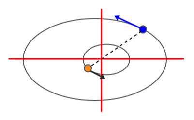
Fig. 11.3 Kepler revisited.

Now that we have seen how to deal with the two-body problem, we can return to the motion of the Earth around the Sun. This is obviously not a two-body problem, but a many-body problem with many planets.

However, we can approximate it to a two-body problem: we ignore all other planets and leave only the Sun and Earth. Hence, there are no external forces. Consequently, the CM of the Earth-Sun system moves at a constant velocity. And we can take the CM as our origin.

We have to solve the reduced mass problem to find the motion of both the Earth and the Sun:

\[ \mu \frac{d^2 \vec{r}_{12}}{dt^2} = -\frac{Gm_e m_s}{r_{12}^2} \hat{r}_{12} \]

Note: this equation is almost identical to the original Kepler problem. All that happened is that \(m_e\) on the left hand side got replaced by \(\mu\).

Everything else remains the same: the force is still central and conservative, etc.

11.5.1. Where is the CM located?

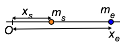
Fig. 11.4 Position of CM in the sun-earth system.

We can easily find the center of mass of the Earth-Sun system. Chose the origin on the line through the Sun and the Earth (see Fig. 11.4).

\[ R = \frac{m_s x_s + m_e x_e }{m_s + m_e} = x_s + \frac{m_e}{m_s + m_e} (x_e - x_s)\approx x_s + 450km \]

In other words: the Sun and Earth rotate in an ellipsoidal trajectory around the center of mass that is 450 km out of the center of the Sun. Compare that to the radius of the Sun itself: \(R_s = 7 \cdot 10^5\) km. No wonder Kepler didn’t notice. The common CM and rotation point is called the Barycenter in astronomy.

11.5.2. Exoplanets

However, in modern times, this slight motion of stars is a way of trying to find orbiting planets around distant stars. Due to this small ellipsoidal trajectory, sometimes a star moves away from us, and sometimes it comes towards us. This moving away and towards us changes the apparent color of the emission of molecules or atoms by the Doppler effect. It is a periodic motion, which lasts a ‘year’ of that solar system. Astronomers started looking out for periodic changes in the apparent color of the light of stars. One can also look for periodic changes in the brightness of a star (which is much, much harder than looking at spectral shifts of the light). If a planet is directly between the star and us, the intensity of the starlight decreases a bit.

And ….. astronomers found one, and another one, and more and hundreds. Currently, more than 5,000 exoplanets have been found.

• Changing color of star light due to a period motion induced by a planet orbiting the star (movie from NASA ).

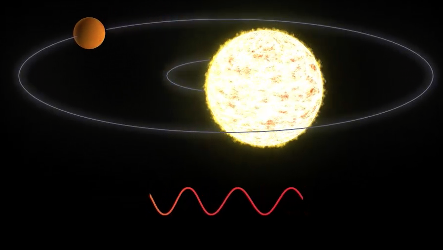
Fig. 11.5 Finding planets via periodic changes in the velocity of a star (from NASA).

• Changing intensity of star light due to a period passage of a planet orbiting the star ((movie from NASA).

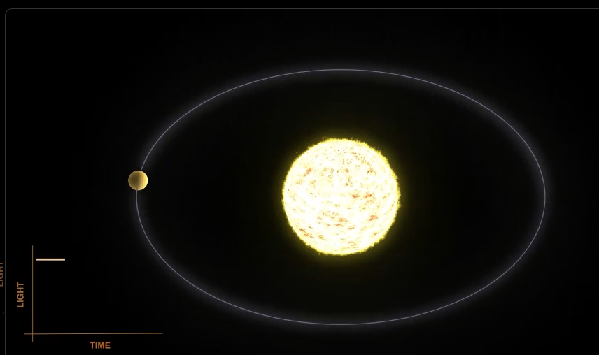
Fig. 11.6 Finding planets via a periodic change in intensity of a star (from NASA).

• Changing intensity of star light due to a period passage of more than one planet orbiting the star (movie from NASA).

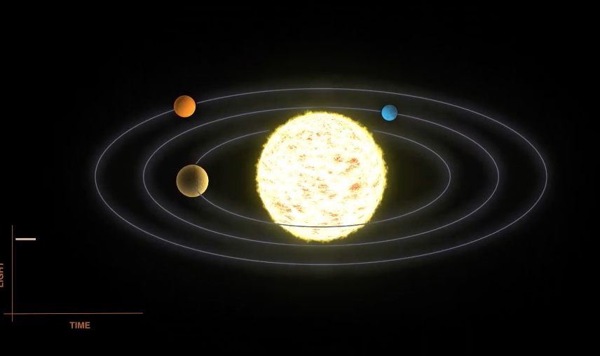
Fig. 11.7 Finding multiple planets via a change in intensity of a star (from NASA).

11.6. Exercises

Exercise 11.1

In the Rutherford scattering analysis, we implicitly used only the mass of the \(\alpha\)-particle when considering the momentum change \(\Delta p/p\). Would it have been correct to use the reduced mass then? If yes, redo the analysis with the reduced mass.

11.7. Three body Problem

Now that we have reduced a two-particle system to a single particle problem, the question arises: can we repeat this ‘trick’ and turn a three-body problem in a two body problem, that in its turn can be reduced to a single particle problem?

The answer is: no. There is no general strategy to reduce a three body problem two a two body-one.

The three body problem is an old one. Already Newton himself worked on it. Its importance stems e.g. from navigation on see. It would be of great help if the position of the moon could be predicted in advance with great accuracy. Then sailors in the 17\(^{th}\), 18\(^{th}\) and 19\(^{th}\) could have found much better their position at full sea. But no one succeeded in providing a closed solution in basic functions.

The king of Sweden, Oscar II, announced, as celebration of his 60\(^{th}\) birthday, a competition with the price awarded to the one that came up with a general solution. But it took a different course. The price went to the French mathematician and physicist Henri Poincaré.

Fig. 11.8 Click here for the Wikipedia page of Poincaré.

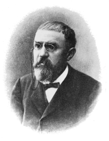
He showed that it was impossible to find such a solution as he reached the conclusion that the three body problem showed chaotic features. It led Poincaré to develop a whole new field: dynamic systems and what we call now deterministic chaos.
The work of Poincaré was the trigger of yet another ‘revolution’ in our understanding of the universe.

It doesn’t mean that there are no known solutions of specific cases of the three body problem. On the contrary, in the movie below 20 solutions are given. Notice that they all have a high degree of symmetry.

Fig. 11.9 Click here to see some exact solutions of the three body problem by Perosello, CC BY-SA 4.0.

11.7.1. Alpha Centauri A, Alpha Centauri B and Alpha Centauri C

The three body problem can also be studied by numerical means. As the equations of motion are easily set up and put into a computer code, this allows us to investigate for instance the three stars of the Alpha Centauri system: Alpha Centauri A, Alpha Centauri B and Alpha Centauri C. This system is a little over 4 million light years away from us: these stars are our closest (star) neighbors. Although it forms a three body system, it is stable due to the much smaller mass op Alpha Centauri C compared to the other two. Alpha Centauri A and Alpha Centauri B are of similar mass, that is 1.1 and 0.9 the mass of our sun, respectively. Alpha Centauri C, on the other hand has a mass of only 0.12 of that of the sun.

Gaurav Deshmukh has written a nice python-based web-page on this system. Below we show some examples of the simulations, that you can do yourself with the code given by Deshmukh.

First, we ignore Alpha Centauri C and used that A and B have about the same mass. The two stars start rotating around each other in ellipsoidal orbits, as we already know from the two body problem.

Fig. 11.10 Alpha Centauri A and B circling each other.

Then, we add a third small one object (not Centauri C, but one with a much smaller mass): \(m_A\) = 1.1, \(m_B\) = 0.907 (both actual relative masses), \(m_C\) = 0.001.

\(m_C\) tries to orbit its closest star, but at some point comes under the influence of the second star and gets ‘tossed around’.

Fig. 11.11 Alpha Centauri A and B circling each other with a third object.

If we let the simulations run for a much longer time, we see that at some point the conditions for our small star are such that it is ‘shot’ into space and disappears for ever.

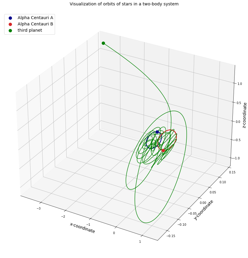
Fig. 11.12 Alpha Centauri A and B circling each other with a third object. The third ‘planet’ is finally escaping into space.

Note: this is a chaotic system and computations need great care.