Decision Analysis#
Decision analysis, or decision-making under uncertain conditions is part of everyday life: when choosing to buy a lottery ticket or choosing to take an umbrella during cloudy weather. In contrast to the rather intuitive decision making in everyday matters, a structured analysis of different alternatives with associated risks, costs and benefits is very useful for decisions in (civil) engineering. This chapter offers a very basic introduction into the decision theory with applications to decision problems in the civil engineering domain. Further reference is made to the work by other scholars for more rigorous and detailed treatment of this topic. See, for example Raiffa and Schlaifer (1961); Benjamin and Cornell (1970).
Introduction#
Making a decision is in fact choosing from alternatives. The decision theory is based on the classic “Homo Economicus” model assumes that the decision-maker:
has complete information about the decision situation;
knows all the alternatives;
knows the existing situation;
knows which advantages and disadvantages each alternative provides, be it in the form of random variables;
strives to maximise that advantage (formally called utility).
The decision-making concept discussed in these lecture notes assumes this model, although decision-making in practice is often different since the above conditions are often not fulfilled. For example, there can be multiple decision makers and multiple objectives, and in reality the decision maker does not know all the alternatives or their outcomes. For many practical cases this has led to an extension of the decision model, but not to a fundamental adjustment of the classical model described here.
Within a decision problem the following characteristics can be distinguished:
the set of all possible actions or decisions \(a\), from which the decision maker can choose
the set of all (natural) circumstances, \(\theta\) that influence the outcomes*
the set of the set of all possible results, \(\omega\), which are functions of the actions and circumstances: \(\omega = f(a,\theta)\).
The actions, natural circumstances and the outcomes can be shown in a so-called decision tree (Figure Fig. 20).
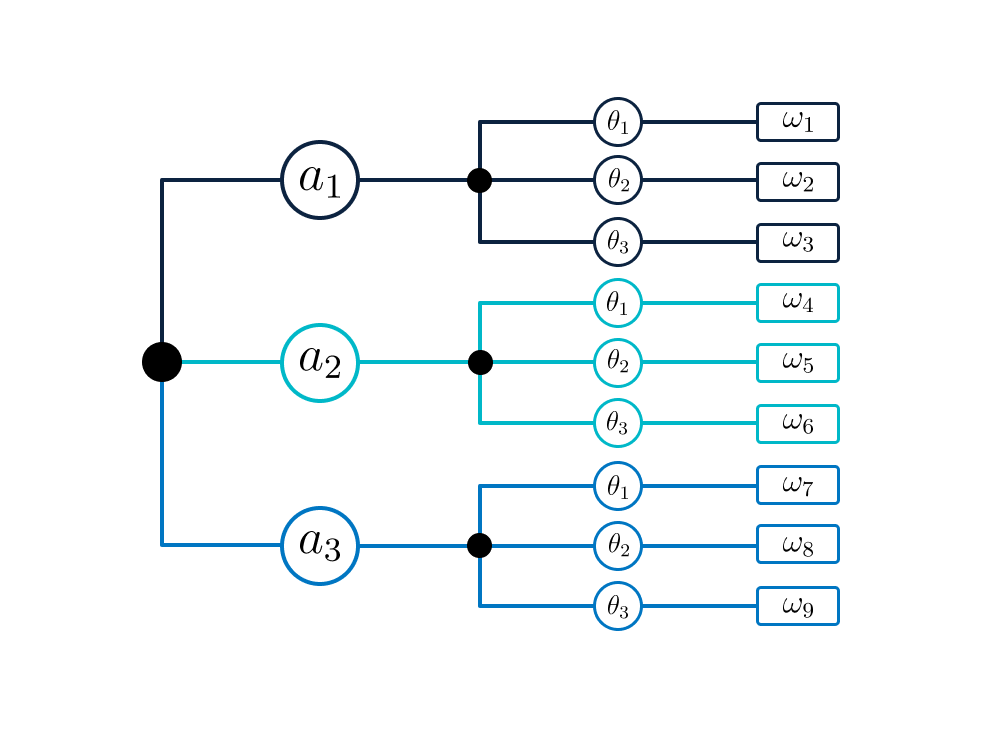
Fig. 20 Decision tree.#
Based on the possible results a choice is made for an action. To be able to assess the different results, a numerical value is assigned to each outcome, \(\omega\), which can be used to establish the benefit of each outcome. This number can be a monetary value, a number on an arbitrary scale or utility–as long as the decision maker(s) can establish a consistent ranking of the outcomes with it. In the last two cases the benefit has no absolute value, but only gives the relative value of the different outcomes.
Utility, \(u\), is a concept used to rank the possible outcomes according to the preferences of the decision maker, with possible values \(0\leq u \leq 1\) . A utility function can be used to characterize the relative utility of various outcomes. The elaborations below are based on the monetary values as a measure for the outcomes and assume a risk neutral decision maker. This is a decision maker who is indifferent between choices with equal expected outcomes, even if one choice is riskier than the other. For example, a risk neutral decision maker would have the same preference for a € 400 pay out, or a 50/50 bet with a coin toss with outcomes of € 0 (head) or € 800 (tail). Utility and risk aversion are further discussed in ater sections.
Decision rules#
Once a set of actions, circumstances and outcomes is known, various approaches can be used to come to a preferred decision. Various deterministic decisions rules are available which do not take into account the probabilities of the possible circumstances and outcomes. One example of such a decision rule is the minimax criterion: a decision maker wants to minimize maximum losses. This is in fact a risk-averse criterion. Another example is the maximax criterion: a decision maker chooses the option with the maximum income and is risk seeking.
Although these decision rules are helpful in some cases, the probability of occurrence of certain circumstances is a key feature of the decision problem. Information on the probability of outcomes is needed for an optimal choice of action(s). For example, when making a decision to start a business in soup or ice cream, the decision maker would want to know what the probabilities of rainy or sunny weather are. Selling ice cream in Dutch winter will probably not make a good (expected) profit, but it would be a profitable business in a Mediterranean summer.
Therefore it is necessary to include information on the probabilities of circumstances and outcomes, in order to determine a rational action with the highest expected value of the benefit. This theory is known as the Bayesian decision theory. In a probabilistic or Bayesian decision framework the optimal action \(a*\) is defined as the one maximizing the expected utility. The following formula is found for the case with discrete outcomes.
In which \(u(a, \theta)\) is the utility of action a under circumstance \(\theta\) and \(P(\theta)\) is the probability that circumstance \(\theta_{i}\) occurs.
A rational decision is choosing the action with the highest expected (utility) value or highest benefit if outcomes are expressed in monetary values. This is illustrated in the example below. Note that other examples in these lecture notes will also be based on monetary values.
Example: buying shares or bonds?
Suppose a person has €1000 at his or her disposal and is given the choice to invest this money in bonds or in shares of a given company. It is known that, on a yearly basis, 3 % of the current market value is distributed as interest on the bonds. The dividend of the shares depends on the company’s profit. Suppose that the board of directors have made the following agreements:
for a profit smaller than 5% of the shareholders capital, no dividend is paid; for a profit larger than 5% of the shareholders capital, dividend is paid, the percentage of which corresponds to 3% of the current market value of the shares;
for a profit larger than 10% of the shareholders capital, the dividend corresponds to 6% of the current market value of the shares.
The set of actions A has two elements: \(a_{1}\)= investing in shares AND \(a_{2}\)= investing in bonds
The set or market circumstances N has three elements, namely:
\(\theta_{1}\) = company profit ≤5 %
\(\theta_{2}\)= 5 % < company profit ≤ 10 %
\(\theta_{3}\)= company profit > 10 %
Assume the inflation amounts to 2 %. The set of outcomes ω contains three possible outcomes for the shares: \(\omega_{1}\)= return (0 % -2 %) = -2 % per annum \(\omega_{2}\)= return (3 % -2 %) = 1 % per annum \(\omega_{3}\)= return (6 % -2 %) = 4 % per annum
Note that for the bonds the net outcome always yields \(\omega_{2}\) =1% (i.e. 3% interest – 2% inflation). The outcomes can be illustrated using a decision tree (see Fig. 21) or a table (see Table 4).
Market circumstances |
|||
|---|---|---|---|
Actions |
\(\theta_{1}\) |
\(\theta_{2}\) |
\(\theta_{3}\) |
\(a_{1}\): buy shares |
\(-\)2 % |
1 % |
4 % |
\(a_{2}\): buy bonds |
1 % |
1 % |
1 % |
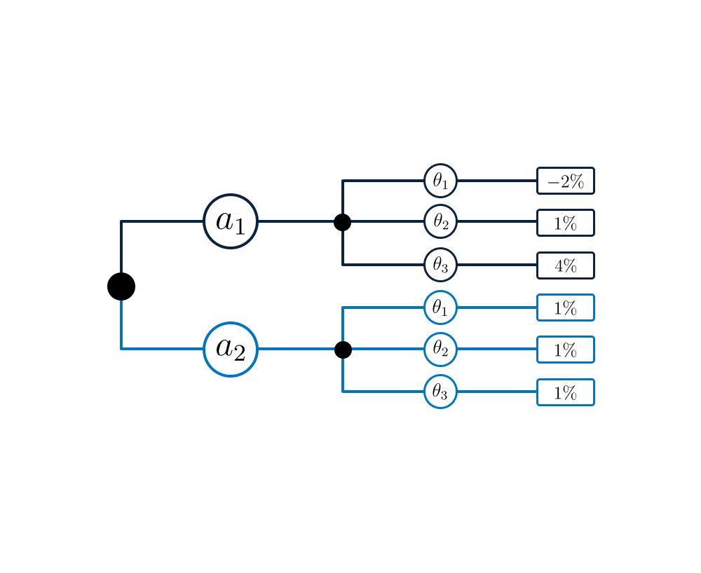
Fig. 21 Decision tree for the example of buying shares (\(a_{1}\)) or bonds (\(a_{2}\)).#
The deterministic decision rules can be applied to this example. Minimax would result in investing in bonds (\(a_{2}\)), maximax would result in buying shares. The optimal decision can be found by taking into account the probabilities of the market circumstances. These three circumstances are assumed to be exhaustive and mutually exclusive (i.e. outcomes cannot overlap and the sum of probabilities equals 1). The probabilities are estimated at \(P(\theta_{1})\) = 0.2; \(P(\theta_{2})\) = 0.3; \(P(\theta_{3})\) = 0.5. These probabilities can now be included in the decision tree. The expected value of the return of the actions is as follows:
Buying shares: 0.2(-2 %) + 0.3 (1 %) + 0.5 (4 %) = 1.9 %.
Buying bonds: 1%
In this case the expected outcome is larger for buying shares than for buying bonds. So for a risk neutral decision maker buying shares (a1) would be the preferred action. Note that this action also includes a probability of 0.2 of a loss. This is also expressed by a higher standard deviation of the expected outcomes for buying shares. The above example can also be extended by applying different utility functions for various outcomes.
In the previous example, the number of circumstances is limited and the probability distribution of the circumstances is discrete. For many decision problems this is not the case. The state of nature, for instance, can assume many values that cannot be made discrete. This, for example, would have been the case if the dividend in example 0 had been a percentage of the profit. In such cases a probability density function can be used to characterize the spectrum of outcomes. Using a continuous form of formula (3.5), the expected value of various actions, and the optimal action / decision can be identified.
In taking decisions with uncertainties, it appears that probabilistic calculation techniques are a valuable aid to reach a rational choice. This is particularly the case if risks are dependent on the possible decisions. In such cases, Bayesian decision theory minimizes the total costs (i.e. investment costs plus risk in terms of potential losses). This can best be illustrated by means of an example from the civil engineering domain.
Example: drainage of a construction site – decision tree
In a river polder a basement has to be built in an excavated construction site. The construction site is made of sheet piling and the bottom is sealed off with a clay layer with a thickness of approximately 2.5 m. The thickness is not known exactly but measurements indicate that a normal distribution can be used with mean \(\mu_d\)= 2.5 m and a standard deviation of \(\sigma_{d}\) = 0.2 m.
The river cuts through the clay layer and the underlying sand layer is fed by the river, which causes high uplift pressures on the clay which is exposed in the excavation (see Figure Fig. 22). If the pressure becomes too high the excavation base will push upward and water will enter the excavation in an uncontrolled way, damaging property and perhaps risking human life.

Fig. 22 Cross-section of excavation and river.#
Measurements of the groundwater levels indicate the maximum upward pressure, \(h\), under the sealing layer in the construction period has an a normal distribution with an expected value of \(\mu_{h}\) = 4 m water column and a standard deviation of \(\sigma_h=0.75 \mathrm{m}\) (see Figures Fig. 23). Since \(h\) is a hydraulic head (units of \([\mathrm{L}]\)), pressure is calculated by multiplying the unit weight of water (\(10\:\mathrm{kN/m^3}\)).
Failure occurs when the uplift pressure exceeds the weight of the clay layer, which can be described by a limit state function \(Z = R - S\) with resistance \(R\) and load \(S\):
Where \(\rho_c\) is the density of clay (\(20\:\mathrm{kN/m^3}\)), and is assumed here to be a deterministic value. The probability of failure is thus \(P(Z<0)\), which for this situation can be found by calculating the mean and standard deviation of \(Z\):
Since \(Z\) also has the normal distribution, we find the failure probability:
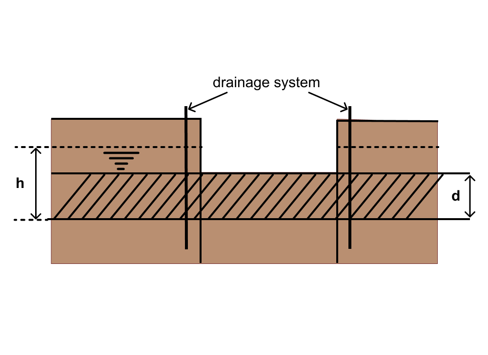
Fig. 23 Cross-section of excavation near a river. Hashed area indicates the clay layer, which is underlain by sand. The water pressure is given by \(h\) and is directly related to the river level (Figure Fig. 22).#
The effect of a drainage system in the construction site (see Fig. 22) on the groundwater levels has been reviewed using groundwater flow calculations. It appears that it reduces the mean value of the maximum water levels to \(\mu _{h}\) = 3.52m and the standard deviation remains the same. In this case the failure probability is reduced to 0.04. Such a drainage system costs €150,000.
The flooding of the construction site will result in estimated damages of €5,000,000, and the designer of the construction site is faced with the choice whether drainage facility is a worthwhile investment. To provide insight, the decision problem is illustrated with a decision tree, but first the set of actions, circumstances and outcomes are defined:
The set of actions A consists of:
\(\textit a_{1}\)= excavation without drainage
\(\textit a_{2}\)= excavation with drainage
The set of circumstances N is formed by:
\(\theta_{1}\)= the sealing layer remains intact
\(\theta_{2}\)= the water pressure exceeds the weight of the sealing layer
The set of outcomes \(\Omega\) consists of:
\(\omega_{1}\) = nothing happens; loss = € 0
\(\omega_{2}\) = the construction excavation is flooded: loss = €5,000,000
The previous analysis has shown that the probability of flooding of the excavation equals \(p_{f}\) = 0.12 for a situation without drainage and \(p_{fd}\) = 0.04 with drainage.
Without drainage, the risk, defined as the expected value of the loss, is
With drainage the risk is:
Costs and probabilities can also be shown in the decision tree (see Figure Fig. 24). The expected values of the costs can be calculated for the different actions by adding the present values of the cost of actions and risk:
\(\textit a_{1}\) : expected value (additional) costs = risk =€ 600,000
\(\textit a_{2}\) : expected value (additional) costs = extra costs + risk = € 150,000 + € 200,000 = € 350,000
This implies that the construction of the drainage system is rationally speaking the best decision for a risk neutral decision maker.

Fig. 24 Decision tree with probabilities and costs.#