System Reliability#
A structure or system in civil engineering generally consists of a set of components (also called elements). Whereas the previous chapter focused on the reliability of a single component, this chapter addresses reliability analysis for systems that consist of multiple components. The consequences of the failure of a component will depend on the type of system that is considered. In some cases, the failure of a component leads to failure of the whole system (progressive collapse). In other cases (and system configurations) there could be no failure if a single component fails and other components take over the function of the failed one.
The techniques introduced in this chapter essential for carrying out step 3 in a risk analysis: quantitative analysis.
Series and Parallel Systems#
In reliability analysis two types of basic systems can be distinguished: series and parallel (see Fig. 16).

Fig. 16 Series (top row) and parallel (bottom row) systems: the building blocks of system reliability analysis.#
Within a series system, failure of a single component will always lead to the failure of the entire system. An example is a chain, which breaks if any individual link fails. In our flood management example, a dike ring protecting a single area that is made up of multiple segments is also a series system. Within a parallel system, failure of one component can be compensated by the performance of another component; it represents the concept of redundancy. Drawing on the chain example, it would imply using more than one chain capable of holding the maximum load. An example from flood management would be to build a second dike ring inside the first dike ring. In practice, a complex system can generally be represented by means of a combination of parallel and series subsystems, just as the parallel system of multiple chains (or dikes) is a parallel system of series systems of links (or dike segments).

Fig. 17 Example of series (top row) and parallel (bottom row) systems, illustrated with a chain and dike ring. Each component in the parallel case is itself a series system: links in the chain and dike segments in the dike ring.#
Systems are often schematized using a system diagram, as in Fig. 16. This also illustrates the function of a system as an input-output diagram, where one can considers the ability to travel from left to right on the figure. It is analagous to many scenarios involving flow: electricity (Fig. 18), water in pipes or transportation routes.

Fig. 18 Series (left) and parallel (right) systems illustrated as a string of lightbulbs.#
Definition of Failure#
Whereas in component reliability problems we defined failure using a function of random variables, in system reliability problems, we define failure based on the continuity of the system diagram. Failure occurs when we are not able to travel from left to right on the diagram due to one or more broken links.
Reliability Calculations#
Equations for computing parallel and series system reliability are described here with the notation \(F_i\) and \(\bar{F_i}\) to denote failure and non-failure of component \(i\), respectively. A system is made up of \(i=1,...,n\) components where the probability of failure of component \(i\) is \(P(F_i)\). Note that as a concept, “system reliability” is almost always going to be quantified using the failure probability of the system, \(p_{f,sys}\). This is sometimes misleading or confusing because the mathematical definition of reliability is the complement of reliability, \(1-p_{f,sys}\).
Parallel System#
A parallel system is often described as redundant since all components must fail to cause system failure. This is also simple to calculate as it can be described mathematically as the joint failure probability, or intersection, of all components:
If the components are independent, this becomes
Although we will not quantify the effect of dependence in depth here, it is easy to see semi-quantitatively that positive dependence increases the intersection probability, and therefore also increases \(p_{f,sys}\). Negative dependence has the opposite effect. In fact, if parallel components are mutually exclusive the system is guaranteed to survive. The case of negative dependence is trivial in engineering reliability computation, but something that is used to motivate the incorporation of resilience or robustness in our risk reduction decisions.
Series System#
A series system fails if any component fails, which is
For two components this can easily be re-written as
Although it is straightforward to write out terms for 3 or more components, it is easier to re-write the union formulation as the complement of joint survival of the system:
As \(\bar{F}_i=1-F_i\), we arrive at the following simple relationship:
The influence of dependence on a series system is most easily understood through consideration of (3), which allows a direct analogy to the parallel case through the intersection term. With positive dependence, the system failure probability decreases
Quantification of Dependence#
Fig. 19 quantifies the effect of dependence on the join probability of failure of two components. The joint failure probability is calculated using the multivariate normal distribution which has a linear dependence measure, the correlation coefficient, \(\rho\). The blue line shows the series system failure probability, equivalent to (3). The figure allows one to evaluate the quantitative effect of dependence on series and parallel systems, and even illustrates the bound of \(p_{f,sys}=P(F_1)\) for the case of \(\rho=+1\).
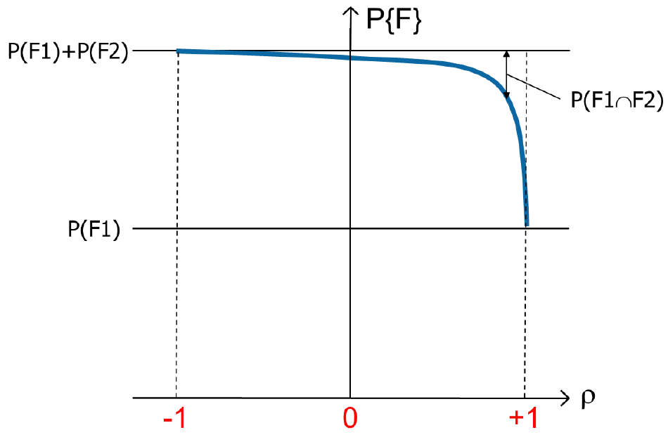
Fig. 19 Effect of correlation coefficient on failure probability for a series system via joint failure, \(P(F1 \cap F2)\) (computed with a Gaussian copula). The arrow is located at \(\rho=+0.9\), where \(P(F1 \cap F2)=0.003\).#
Tips for Interpreting the Figure
Fig. 19 is interesting because it shows the effect of dependence on both series and parallel systems, since they are related with (3), the value that is shown in the blue line. Note that the distance between the blue line and the top reference line is the value of the intersection, \(P(F1\cap F2)\) (also called the “joint” or “and” probability). Note that without a joint probability distribution (in this case a bivariate Gaussian), you can’t compute the joint probability of two events, except for three special cases, the vertical black lines in the figure—do you know what those values are? This is related to the concepts of dependent, mutually exclusive and statistically independent events, which are easy to confuse with each other.
It is also common to think about dependence in the sense of how “one event happens given that the other event has happened,” but this is not quite right. Dependence is describged simply by the definition of conditional probability
which means the correct statement is that dependence quantifies how the “probability of one event changes (or not) given that the other event has happened.”
Chapter Overview#
This page contains a brief introduction to the computation of failure probability for series and parallel systems, and describes the role of dependence. The following section illustrates these concepts with a simple exercise.
Additional Information#
The word ‘system’ in the title of this chapter refers to a reliability analyses made up of more than one distinct components. It may or may not be the same as the system for which the risk analysis is being done. For example, in the flood risk case we look at a dike ring, which is a series system of dike segments. Each dike segment can fail in a variety of ways (e.g., sliding or eroding), where if any of these types of failure occurs, the dike fails; a series system. Thus, the dike ring is a series system, where each component also a series system.
System reliability analysis can look very similar to component reliability problems, especially when various combinations of discrete and continuous random variables are incorporated. In reality, all of these problems are generalized by the concept of a multivariate probability distribution. The concepts are separated following conventions in engineering practice, as well as for the convenience of illustrating analytic and numerical solutions.
The primary author for this chapter is Robert Lanzafame.