Component Reliability#
This Section gives a brief introduction to some of the mathematical foundations of component reliability theory, which is focused on determining the probability of a ‘bad thing’ happening (see Risk and Reliability for Engineers). The topic has also been covered in the Probabilistic Design Section (especially the Two Random Variables example), and is a key part of Step 3 (quantitative analysis) in the Steps in a Risk Analysis.
Definition#
In short, a component reliability analysis evaluates the reliability of a particular engineered object, where reliability is the complement of failure probability, \(p_f\). The analysis is performed by defining a function of random variables, \(g_X(x)\), and mathematically specifying a region of interest, \(\Omega\), often called the failure region. The function of random variables implies a multivariate probability density function, \(f_X(x)\), where integrating over the failure region \(\Omega\) gives \(p_f\).
A Simple Case#
The most simple reliability analysis is a univariate case with one random variable. Consider a water distribution system that relies on groundwater (i.e., one component within the system). Suppose we can model the groundwater elevation as a random variable with the normal distribution:
If \(h_w\) drops below 2 m, the pumps run dry, and our component fails. In this case our function of random variables is simply:
and failure is defined as:
The component reliability analysis is thus:
Which is easily evaluated with the CDF of \(h_w\):
This is nearly equivalent to the One Random Variable example using river discharge from the Probabilistic Design Chapter, the only difference is there a load variable was considered and therefore evaluated with the complementary CDF.
Not Simple Cases#
The example above is ‘simple’ for three reasons, specifically. It has:
only one random variable, so the distribution of \(g(X)\) is also univariate
the function of random variables, \(g(X)\) is linear
the distribution of the random variables (variable, in this case) is Gaussian
These three characteristics make component reliability problems very easy to solve. In fact, you should have already done this earlier probability courses with (co)variance propagation methods. For example, solving for the mean and standard deviation of a linear function of random variables that are each Gaussian is straightforward, as the function of random variables is also Gaussian. Unfortunately, as problems become more complex, so do the methods required for solving such problems.
In this book we focus on simple situations with up to two variables (the ‘bivariate’ case) that can be solved analytically (linear functions and Gaussian random variables). Random variables are limited to continuous parametric distributions and linear measures of dependence (correlation coefficient, multivariate Gaussian). If these requirements are relaxed, we will use simulation to calculate the failure probability numerically (i.e., Monte Carlo simulation).
With this in mind, a generic procedure for using component reliability analysis in a probabilistic design context is:
determine probability distributions for each random variable (marginal distributions)
specify dependence between random variables (or independence)
define the function of random variables, \(g_X(X)\), and region of interest, \(\Omega\)
integrate multivariate PDF, \(f_X(X)\), over \(\Omega\) to evaluate probability of interest
check probability requirement, and if needed:
modify component (i.e., modify 1, 2 or 3)
repeat 4, 5 and 6 until the requirement is met
Note
The term ‘failure’ here, widely used in civil engineering, is used here as a matter of convenience. Component reliability methods can also be used to find the probability of something that has nothing to do with failure, as long as it can be desribed with a function of random variables.
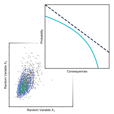
Two Random Variables#
The example with discharge from two rivers in the Probabilistic Design Chapter can be considered a component reliability problem with two random variables. The discharge of both tributary rivers act as loads because they both are proportional to the main design variable, \(q\) or \(h_{dike}\). The reliability integral is thus
where the failure region \(\Omega\) contains all values of \(Q_1\) and \(Q_2\) such that the river level exceeds the dike height:
Note that if the dike were constructed to a height of 8.29 m, the component reliability would be 0.01 and the failure region would be equivalent to Fig. 7.
The primary author for this chapter is Robert Lanzafame.