import matplotlib
if not hasattr(matplotlib.RcParams, "_get"):
    matplotlib.RcParams._get = dict.get
Contaminant Transport#
import numpy as np
import matplotlib.pyplot as plt
from scipy.special import erfc
from scipy import stats

from exercise_setup import process_negative_values
from exercise_setup import RandomVariableDistribution
from exercise_setup import pdf_of_function_of_RV
from exercise_setup import monte_carlo
Interactive Python Page
The code on this page can be used interactively: click –> Live Code in the top right corner, then wait until the message Python interaction ready! appears.
When this page is activated:
Several packages will be imported automatically
Code cells will not be executed automatically (you do it!)
The download button provides a *.zip file with everything needed to run this analysis on your computer.
Which packages are imported when this page is activated?
import numpy as np
import matplotlib.pyplot as plt
from scipy.special import erfc
from scipy import stats

from exercise_setup import process_negative_values
from exercise_setup import RandomVariableDistribution
from exercise_setup import pdf_of_function_of_RV
from exercise_setup import monte_carlo
Here we use component reliability methods to evaluate the probability of a contaminant causing dangerous concentrations in a groundwater well. The contaminant plume is transported on the groundwater phreatic surface due to advection and diffusion.
The purpose of this exercise is to:
evaluate component reliability
illustrate functions of random variables
see the effect of random variable distributions on reliability
consider ‘sensitivity’ as a functional and/or stochastic influence on the limit-state function
Instructions for Interactive Programming Exercise#
This page is designed to lead you through the analysis sequentially, so we recommend executing the cells one-by-one as you read through the page. Afterwards, you are welcome to use the “run all” button to execute all cells on the page.
Once the interactive feature is activated, you can use the code cells to answer the following questions:
Which random variables have the biggest influence on reliability?
How does the assumption of probability distribution influence reliability?
Do the random variables act as loads or resistances?
Introduction of Case Study#
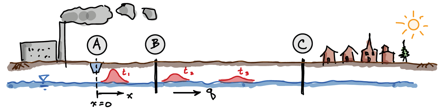
The case study is a contaminant transport problem, illustrated in the figure below. A factory located near a town produces hazardous waste, which can threaten the drinking water supply of the town that is extracted from groundwater wells (C). The regional groundwater system has a gradient that causes water to flow in the direction of the town from the factory, thus any spilled hazardous waste that enters the ground will eventually be transported to the wells. In order to mitigate the consequences of a spill a ditch is constructed around the factory to collect it (A). Unfortunately, even with powerful pumps, there will still be some waste that reaches the groundwater table. Our task is to quantify the probability that the waste concentration exceeds the maximum exposure level to prevent the drinking water becoming unhealthy.
Contaminant Transport#
Once the ditch becomes contaminated it is cleaned quickly, but unfortunately a ‘pulse’ of contamination enters the ground, after which the regional gradient carries it towards the town (advection). The pulse also disperses due to diffusion, which results in a classic advection-diffusion problem (see red shapes in diagram, at three different times, \(t\)). Because the ditch extends a long distance in the lateral direction and the contaminant is buoyant (it floats on the groundwater table and we neglect vertical dispersion), the problem can be analyzed in 1 dimension with the following analytic expression:
Where \(C\) contaminant concentration (e.g., parts per million, ppm) at distance \(x\) from the ditch at time \(t\) after the spill, and \(C_0\) is the concentration in the ditch (just prior to cleanup). \(\mathrm{erf}\) is the error function. There are three parameters in the equation which are related to soil properties and groundwater flow:
\(q\) is the horizontal groundwater flow velocity (specific discharge) [m/day]
\(n\) is the soil porosity [\(-\)]
\(a\) is the longitudinal dispersivity, which describes dispersion in the left to right direction in the image [m]
Unfortunately there is not a lot of soil information, so we have to take into account uncertainty in these three variables, using the following probability distributions with first and second moments (i.e., \(\mu\) and \(\sigma\)).
\(q\sim\mathrm{N}\left(\mu_q=1.00,\sigma_q=0.10\right)\)
\(n\sim\mathrm{N}\left(\mu_n=0.20,\sigma_n=0.02\right)\)
\(a\sim\mathrm{N}\left(\mu_a=10.0,\sigma_a=1.00\right)\)
It is important to check the sensitivity of the reliability analysis to the distribution type and moments. We will use the concentration ratio \(C/C_0\) to evaluate this problem and compare it to a threshold defined by health regulations: \(\mathrm{threshold}=1e-4\).
Definition of Limit States#
As shown in the figure above, there are two locations of interest: the monitoring station (\(x=100\) m from the ditch, point B) and the town well (\(x=500\) m, point C). We are interested in evaluating two cases with a reliability analysis:
Whether the contamination can be detected at the monitoring station above the threshold level within 1 week of the spill, and
If the contamination level at the town groundwater well exceeds the threshold level within 1 month of the spill (30 days)
Relating these descriptions to our variables of interest:
find the probability that \(C/C_0\) > threshold
find the probability that \(C/C_0\) < threshold
We will refer to these values as ‘failure probabilities’, even though case 1 technically doesn’t correspond to failure—it’s just the way we refer to things in practice.
Next we will convert these into functions that will allow us to quantify the ‘failure’ conditions. For convenience, it is often useful to define the limit state as a function, \(Z\), such that failure occurs when \(Z<0\). It follows from the descriptions above, that the limit state functions for both cases are:
\(Z=C/C_0 - \mathrm{threshold}\)
\(Z=\mathrm{threshold} - C/C_0\)
NB: in the book another notation used for \(Z\) is \(g_X(X)\).
Analysis Approach#
Our programming task is to create a function of random variables to represent these two limit-states, define the random variables, then evaluate the reliability with Monte Carlo simulation. In other words, we will numerically approximate the probability distribution of \(Z\), then evaluate reliability as \(P(Z<0)\).
This is a lot of work, but fortunately a number of helper functions and a Class are provided in the auxiliary file exercise_setup.py!
References#
This example draws inspiration from Case 2 of the paper by Sitar et al. (1987).
Defining the Limit States#
We only define limit state Case 2 below, and will use a simple multiplying factor of \(-1\) to switch to Case 1 using a multiplying factor flip_LSF.
def C_C0(q, n, a, x, t):
    """Contaminant concentration ratio."""
    q, n, a = process_negative_values(q, n, a)
    return 0.5*erfc((x - q/n*t)/(2*np.sqrt(a*(q/n)*t)))

def limit_state_fun(q, n, a, x, t, threshold):
    """Limit state fxn, Case 2 (multiply by flip_LSF=-1 for Case 1)."""
    return threshold - C_C0(q, n, a, x, t)
Class RandomVariableDistribution#
The class RandomVariableDistribution makes it very easy to define Normal and Lognormal distributions for the random variables. See documentation and example below.
NB: you can use the code in exercisesetup.py and this notebook to confirm the result of the 2 random variable case in the Probabilistic Design chapter, and recreate the figures.
print(RandomVariableDistribution.__doc__)
example_random_variable = RandomVariableDistribution()
example_random_variable.define_distribution(mean=5,
                                            dist_type='LN',
                                            print_new_dist=True)
example_random_variable.plot_pdf_or_cdf()
Setting up the problem#
N = 10000

t = 7
x = 100
threshold = 1e-4

flip_LSF = -1

q_rv = RandomVariableDistribution()
q_rv.define_distribution(mean=1., stddev=.1)
n_rv = RandomVariableDistribution()
n_rv.define_distribution(mean=0.2, stddev=.02)
a_rv = RandomVariableDistribution()
a_rv.define_distribution(mean=10., stddev=1.)
Monte Carlo analysis#
The Monte Carlo procedure for estimating failure probability, \(p_f\), is:
For each random variable \(X_i\) (\(i = 1, …, n\)) one simulates N realizations, \(x_{i,1}, x_{i,1}, ..., x_{i,N}\).
For each set of simulations \(j\) (\(j = 1, ..., N\)) one calculates \(g(x_{1,j}, x_{2,j}, …, x_{n,j})\)
In case \(g(.) < 0\) a counter \(N_f\) is increased by one. After \(N\) simulations one calculates: \(\hat{p}_f=N_f/N\)
In case \(N\rightarrow+\infty\) one obtains the failure probability \(p_f\).
The number of simulations \(N\) directly influences the accuracy of \(\hat{p}_f\), which is an estimate of the ‘true’ value \(p_f\). As an infinite number of simulations is not possible, one must choose a value for \(N\) that balances total computation time, which increases linearly with \(N\), and accuracy of the estimator \(\hat{p}_f\), which can be determined as the number of significant digits desired for \(p_f\), or based on relative error (coefficient of variation, \(V=\sigma/\mu\). The failure observations, \(N_f\), within the Monte Carlo procedure are the result of a sequence of statistically independent and identically distributed random trials in a Bernoulli process. Using the binomial distribution, the standard deviation of \(\hat{p}_f\) can be written
As \(\hat{p}_f\rightarrow1\) this leads to the coefficient of variation, \(V_{\hat{p}_f}\):
The coefficient of variation is a useful measure for gauging the accuracy of a Monte Carlo simulation: values of 0.01 are ideal, but 0.1 can be sufficient in many applications, depending on the need for accuracy. For example, consider \(V=0.1\) for a target failure probability of \(0.01\). Assuming the samples follow a Gaussian distribution implies a probability of 0.997 that the ‘true’ failure probability is within the interval 0.007-0.013. It is also useful to plot the calculated values of \(V\) and \(\hat{p}_f\) for every realization \(j = 1, ..., N\), as shown below. The figure clearly shows convergence to a stable value of \(\hat{p}_f\) after X simulations, indicating that for future analyses that are similar can use a lower number of simulations instead (\(N\sim X\)).
In case of a target coefficient of variation the number of required simulations \(N\) increases as \(p_f\) decreases. As an example, for \(V = 0.01\) and \(p_f=1e-5\) one has to execute \(10^9\) simulations. As for this case on average only one of \(10^5\) simulations leads to an increase of \(N_f\), the frequency of obtaining a ‘success’ (realization in the unsafe domain) is very low. In addition, for low failure probabilities the number of function evaluations is quite high, which may be practically impossible if there is a high function evaluation time, for example with a complex finite element model. To address this problem, variance reducing techniques have been developed which allow the simulations to be performed in a more effective way. In the following the so-called importance sampling or Latin hypercube sampling.
sample_q = q_rv.get_sample(N)
sample_n = n_rv.get_sample(N)
sample_a = a_rv.get_sample(N)
sample_C_C0 = C_C0(sample_q, sample_n, sample_a, x, t)
sample_Z = flip_LSF*limit_state_fun(sample_q,
                                    sample_n,
                                    sample_a,
                                    x, t, threshold)

monte_carlo(sample_Z);
The method pdf_of_function_of_RV makes it easy to see what the distribution of \(C/C_0\) and the limit state function for different distributions of q, n or a. Below a second distribution of a is considered:
C_C0_cases = []
Z_cases = []
C_C0_cases.append(sample_C_C0)
Z_cases.append(sample_Z)

a_2 = RandomVariableDistribution()
a_2.define_distribution(mean=10, stddev=4, dist_type='N')
C_C0_cases.append(C_C0(sample_q, sample_n, a_2.get_sample(N), x, t))
Z_cases.append(flip_LSF*limit_state_fun(sample_q,
                                        sample_n,
                                        a_2.get_sample(N),
                                        x, t, threshold))

a_rv.print_status()
a_2.print_status()

pdf_of_function_of_RV(C_C0_cases)
pdf_of_function_of_RV(Z_cases, case_C=False)
This is the density of the function of random variables, \(C/C_0\), two values of \(\sigma_a\), and a third with the uniform distribution (not using the RandomVariableDistribution class).
values_of_RV_1 = sample_q
values_of_RV_2 = sample_a

fig, ax = plt.subplots(figsize=(4, 4))
plt.plot(values_of_RV_1[sample_Z>0], values_of_RV_2[sample_Z>0], 'o',
         markeredgecolor='k', alpha=0.1, markersize=5, color='k')
plt.plot(values_of_RV_1[sample_Z<0], values_of_RV_2[sample_Z<0], 's',
         markeredgecolor='k', alpha=0.7, markersize=5, color='cyan')
ax.set_xlabel('Random Variable 1 (chosen by you)')
ax.set_ylabel('Random Variable 2 (chosen by you)')
ax.set_title('Joint density of 2 RVs with failure realizations')
Case 2: exceeding the health threshold#
Now we return to the failure definition of exceeding the threshold (flip_LSF = 1).
N = 100000

t = 30
x = 500
threshold = 1e-4

flip_LSF = 1

sample_q = q_rv.get_sample(N)
sample_n = n_rv.get_sample(N)
sample_a = a_rv.get_sample(N)

sample_C_C0 = C_C0(sample_q, sample_n, sample_a, x, t)
sample_Z = flip_LSF*limit_state_fun(sample_q,
                                    sample_n,
                                    sample_a,
                                    x, t, threshold)

monte_carlo(sample_Z);
values_of_RV_1 = sample_q
values_of_RV_2 = sample_a

fig, ax = plt.subplots(figsize=(4, 4))
plt.plot(values_of_RV_1[sample_Z>0], values_of_RV_2[sample_Z>0], 'o',
         markeredgecolor='k', alpha=0.1, markersize=5, color='k')
plt.plot(values_of_RV_1[sample_Z<0], values_of_RV_2[sample_Z<0], 's',
         markeredgecolor='k', alpha=0.7, markersize=5, color='cyan')
ax.set_xlabel('Random Variable 1 (chosen by you)')
ax.set_ylabel('Random Variable 2 (chosen by you)')
ax.set_title('Joint density of 2 RVs with failure realizations')
Gradient Vector#
Partial derivatives will be useful for evaluating the functional influence of the variables on the limit states. The gradient vector is defined as:
\(\nabla_{\mathbf{y}} G(\mathbf{y})=\left(\frac{\partial G(\mathbf{y})}{\partial \mathbf{y}_1}, \cdots, \frac{\partial G(\mathbf{y})}{\partial \mathbf{y}_n}\right) \)
To find the gradient vector we need to find the partial derivatives of \(\frac{C}{C_0}\)
\(\frac{C}{C_0} = \frac{1}{2} \mathrm{erfc}\left(\frac{x-(q/n)t}{2\sqrt{a(q/n)t}}\right)=\frac{1}{2} \left(1-\mathrm{erf}\frac{x-(q/n)t}{2\sqrt{a(q/n)t}}\right)\)
Using \(\frac{\partial}{\partial x} (\mathrm{erf} x) = \frac{2}{\sqrt{\pi}}e^{-x^2} \) and \(\Omega = \frac{1}{\sqrt{\pi}}e^{-\left(\frac{x-(q/n)t}{2\sqrt{a(q/n)t}}\right)^2} \), the derivatives are:
\(\frac{\partial (C/C_0)}{\partial x} = \Omega\left(-\frac{1}{2\sqrt{a(q/n)t}}\right)\)
\(\frac{\partial (C/C_0)}{\partial t} =\Omega\left(\frac{x}{4\sqrt{a(q/n)t^3}}+\frac{q}{4n\sqrt{a(q/n)t}}\right)\)
\(\frac{\partial (C/C_0)}{\partial q} = \Omega\left(\frac{x}{4\sqrt{a(1/n)tq^3}}+\frac{t}{4n\sqrt{a(q/n)t}}\right)\)
\(\frac{\partial (C/C_0)}{\partial n} = \Omega\left(-\frac{x}{4\sqrt{aqtn}}-\frac{qt}{4\sqrt{qatn^3}}\right)\)
\(\frac{\partial (C/C_0)}{\partial a} = \Omega\left(\frac{x-q/nt}{4\sqrt{(q/n)ta^3}}\right)\)
def gradient(q, n, a, x, t):
    Om = 1/np.sqrt(np.pi)*np.exp(-((x - q/n*t)/(2*np.sqrt(a*q/n*t)))**2)
    dx = Om*(-1/(2*np.sqrt(a*q/n*t)))
    dt = Om*(x/(4*np.sqrt(a*q/n*t**3)) + (q)/(4*n*np.sqrt(a*q/n*t)))
    dq = Om*(x/(4*np.sqrt(a*q**3/n*t)) + (t)/(4*n*np.sqrt(a*q/n*t)))
    dn = Om*(-x/(4*np.sqrt(a*q*n*t)) - (q*t)/(4*np.sqrt(a*q*n**3*t)))
    da = Om*((x - q/n*t)/(4*np.sqrt(a**3 *q/n*t)))
    return np.array([dq,dn,da,dx,dt])
print(gradient(2.5, 0.2, 10, x, t))
Your turn!#
Now try and use the code to answer the questions posed at the beginning of the notebook, which are repeated here:
Which random variables have the biggest influence on reliability?
How does the assumption of probability distribution influence reliability?
Do the random variables act as loads or resistances?
In particular, to evaluate sensitivity, you can consider two quantitative aspects:
What is the functional influence of the random variables and x and t on the limit-state function?
What is the stochastic influence of the random variables,
What is the combined influence of the two aspects above?