Risk Curve

As introduced in the Definition of Risk Section, the risk curve is useful for evaluating the expected damages for a wide range of scenarios. In contrast to the total expected damages, it allows the comparison of relative magnitude of probability of occurrence and associated consequences. An FN curve tends to be the most widely used, where the ‘N’ refers to number of fatalities and the ‘F’ in comes from the CDF of the probability distribution of \(N\), \(F_N(n)\), although the curve itself actually represents the complementary CDF, \(1-F_N(n)\). It is often plotted on a log-log scale to allow comparison over a wide range of scenarios. While in theory a risk curve can be derived from the probability density function (or probability mass function for discrete cases), the distribution of damages is rarely known and must be approximated by considering a finite and suitable set of discrete events. Thus, in practice, the curve is constructed using scenarios as defined previously in our risk definition (Equation (1)).

Although the FN curve is widely used, the risk curve is not exclusively applied to evaluate expected number of fatalities, \(N\). In principle any measurable quantity can be used to evaluate risk, referred to as a metric, although it can be difficult to apply this to some situations. For example, assessing the value of environmental characteristics can be challenging because the benefit is not easily related to a measurable quantity. The area of impacted wetland habitat during a flood (e.g., km\(^2\)) can be used as a risk metric, but this may not properly represent actual damage, which may recover quickly or slowly depending on the frequency of inundation. Financial damage (e.g., €) is often considered as a risk metric, in which case the FN curve is called an FD curve.

Fatalities and Damages

In some cases it is useful for planning and design purposes to equate \(N\) and \(D\), but this places a specific financial value on human life, which raises difficult moral and ethical concerns. This topic is discussed further in the Valuation of Human Life Section.

A Famous Risk Curve

A risk curve is often useful because it can convey a large amount of complex information in an easily recognizable format. University lectures and conference presentations around the world which focus on risk, especially for civil engineering applications, will often begin with a casual reminder that ‘risk is probability times consequences’ and show some version of a risk curve. Fig. 12 is the most famous risk curve, having been shared widely over the last decades, perhaps because it so nicely compares a wide range of engineering projects.

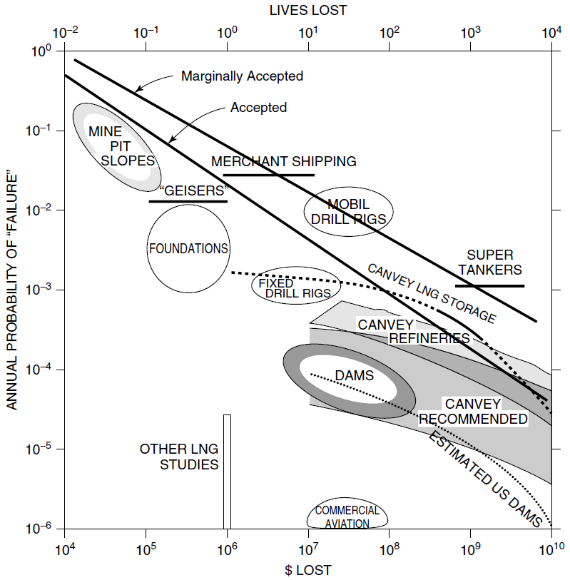
Fig. 12 Risk curve for various engineering projects, showing probability of exceeding a specific number of fatalities, \(N\), and damages, $, on a Log-Log scale, making it both a FN and FD curve; this figure is also included in the Definition of Risk Section. Source: Baecher and Christian (2003), based on Baecher (1982) and described in Baecher (2021).

Fig. 12 was created as part of a risk analysis for a petrochemical storage facility in Tokyo Bay, Japan, where large tanks, constructed on soft soils (hydraulic fill), are vulnerable to damage during an earthquake. Of primary concern was to prevent the petrochemicals entering bay waters, thus not only failure of the storage tanks, but also the containments systems in place to collect spilled material (a complicated system reliability problem). The client needed to convince the regulator that the final design was sufficient for keeping the risk of loss of containment to a sufficiently small level, which the project team was able to do by comparing the risk calculated for the Tokyo site to other engineering works around the world. The figure clearly illustrates what the estimated risk is for each project, and by making the assumption that these already-constructed projects provide a level of safety that is acceptable to society (primarily via regulatory agencies), the ‘acceptable’ line can be used to approve other projects. This concept of acceptable standards based on risk curves is covered in depth in the Section on Safety Standards.

The origin of this figure was described a Terzaghi Lecture by Professor Gregory Baecher, which can be viewed on YouTube: IFCEE 2021: Karl Terzaghi Lecture: Greg Baecher: Geotechnical Systems, Uncertainty, and Risk (Baecher, 2021)}. The introduction to the Tokyo Project begins at 16:16, and the explanation of the risk curve is given at 27:00; however, the entire lecture is well worth listening to and closely related the subject of this book.

Construction of an FN Curve

The following three figures illustrate the computation of an FN curve for a system with two mutually exclusive event scenarios:

• Accident 1 with \(N_{1}=10\) fatalities and a probability of \(P_{1} = 10^{-2}\) per year

• Accident 2 with \(N_{2}=100\) fatalities and a probability of \(P_{2} = 10^{-3}\) per year

First, the probability mass function is created \(f_N(n)=P(N=n)\), taking care that the probability of no fatalities is included:

\[ P(0) = 1 - P_{1} - P_{2} = 1 - 0.01 - 0.001 = 0.989 \]

The cumulative distribution function, \(F_N(n)=P(N\leq n)\), can thus be easily computed, as well as the probability of exceedance, \(1-F_N(n)\), also known as the FN curve. Note that if a risk metric such as damage in Euros was being used, we would call this the FD curve and use \(D\) to denote the random variable, as in \(f_D(d)\) and \(F_D(d)\)

While the curves below illustrate probability and consequences associated with specific scenarios, the expected value of the distribution can be computed, which is equivalent to the area under the FN curve. This is useful can be used to assess the entire system. For this example, the expected value of fatalities per year for all scenarios can be computed as follows:

\[E(N) = P_{1}N_{1} + P_{2}N_{2} = 0.2\quad \textsf{(fatalities per year)}\]

Fig. 13 Probability mass function (PMF), \(f_N(N)\).

Fig. 14 Cumulative distribution function (CDF), \(F_N(n)\).

Fig. 15 Exceedance probability (FN curve), \(1-F_N(n)\).

Practice Exercise

You can practice constructing a simple FN curve in FN Curve, although some of the questions require knowledge of limit lines, introduced in the Safety Standards Section.