6.1. What is AI?#
If you don’t know how AI, and in particular LLMs, work, it may seem like magic - you can give ChatGPT a prompt and it is able to respond quite accurately, typing out the answer in real time and appearding sentient. However, LLMs are not magic but rather a complex multilevel mathematical function. This function contains a huge set of parameters, which are initially set at random. Through training using large data sets, the parameters get tweaked, such that the output of the function improves. The more training the model gets, the better the parameters are and the better output it gives.
6.1.1. Neural networks#
Almost all AIs, including ChatGPT, are based on neural networks. The most important parts of these networks are the neurons that form them. Neurons are simply elements containing a value between 0 and 1. This value indicates how active a neuron is. Zero means that the neuron is “inactive”, whereas one indicates an “active” state.
To build a neural network, one has to simply create and connect layers of neurons. All neurons in one layer are connected to each neuron in the next layer.
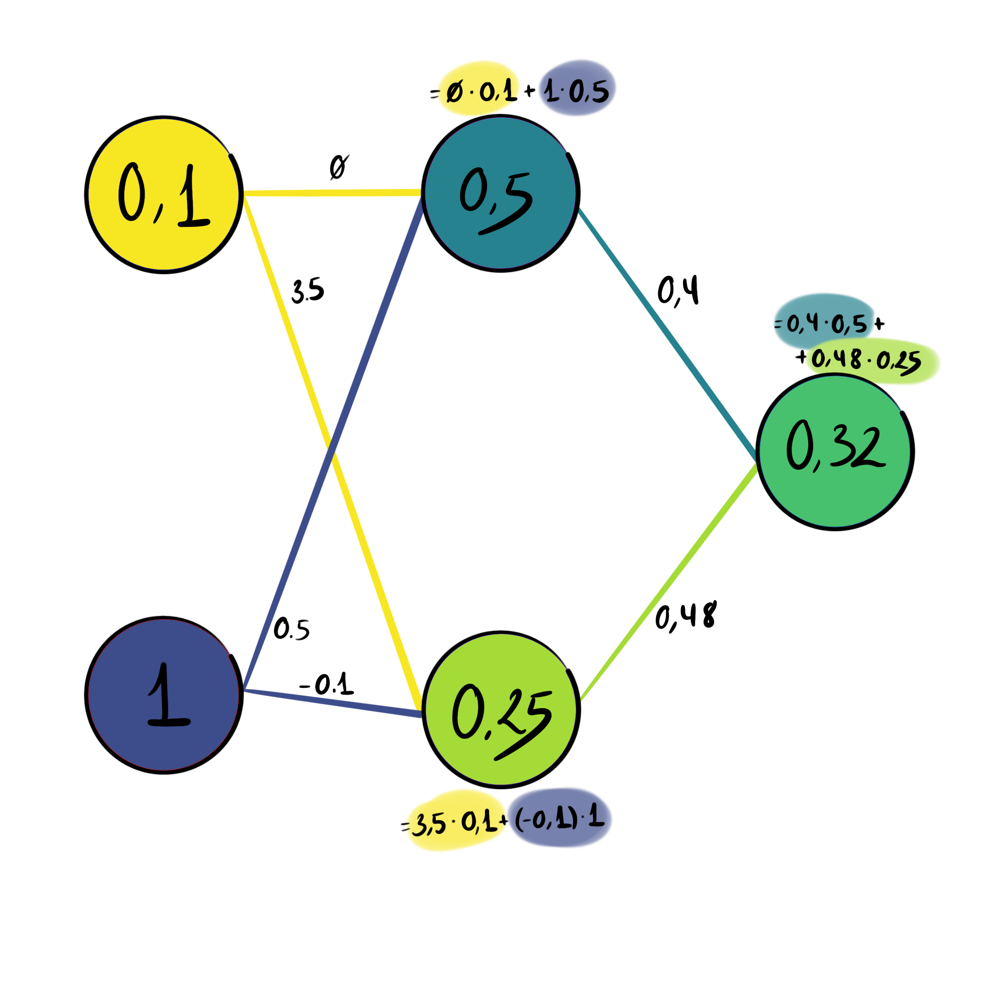
Fig. 6.1 A very simple neural network, made of one hidden layer with two neurons in it. Input layer is on the left and output on the right.#
The first layer is an input layer, consisting of two neurons. This layer contains our input data. For example, for ChatGPT this would be the prompt we give it.
The second layer is the hidden layer. In this example there is only one hidden layer, also with two neurons. These layers contain values that change based on the input and then lead to the desired output.
The final layer is the output layer. This contains all the information that is put out by the neural network. In this example, there is only one output neuron. In the case of ChatGPT, this would correspond to the answer it gives you.
While here we only had one hidden layer, this is a very simplified version - in reality, AI models can use up to thousands of hidden layers with thousand of neurons each. These hidden layers are, as the name suggests, hidden, and they contain operations that alter the input such that we arrive at the desired result in the output layer.
This altering of the input is achieved through the connections between neurons, which affect the state or value of the neuron. Each connection between neurons has a certain weight. This weight will determine how much the neuron in the first layer affects the neuron in the second layer. Mathematically this means that the value of a neuron in the hidden or output layer is just the sum of all values in the previous layer, multiplied by their individual weights. In addition, each neuron has a bias, which offsets its value independently from the previous neurons.
\(w_i\) : The weight of the connection from neuron ( \(i\) ) in the previous layer.
\(a_i\) : The activation (output) of neuron ( \(i\) ) from the previous layer.
\(i\) : Index representing each neuron in the previous layer, with ( \(n\) ) total neurons.
\(B\) : The bias term, which offsets the total value of this neuron.
\(\zeta\) : This a function that serves to control the final value the neuron takes
Activation Functions
Activation functions serve to create complex mappings between model inputs and outputs. While activation functions \(\zeta\) can be a simple linear mapping (\(\zeta(x) = x\)) that won’t change the value at all, you can also choose non-linear activation functions. These can introduce non-linearity to the model, which help neural networks better learn a variety of phenomena.
A neural network is just a function - since a neuron’s value depends on the inputs it receives, we can view each neuron as a function that, given a specific input, consistently produces a certain output. Because a neural network is essentially a collection of these interconnected neurons, it behaves similarly, meaning the entire network acts as a highly complex function.
6.1.2. Training the network with backpropagation#
A necessary step in creating a useful neural network is training the network. Training the network basically means adjusting the weights that connect the neurons. Initially these weights are set randomly. This means that, without training, the weights will remain random and the output of the neural network is nonsensical.
To train the neural network and adjust the weights, we use backpropagation. This basically means that we give an input, let it travel through the neural network and then evaluate the output. Based on this evaluation, we move back in the neural network to slightly adjust the weights, so it makes a tiny bit more sense. Repeating this step continuously with a whole load of data will eventually give you useful weights.
The evaluation is done based on a cost function. The output of the network is compared to the desired output and a cost function evaluates how much they differ from each other. A big difference will result in a high cost. Thus the goal of the backpropagation is to minimize the cost function, which is done by adjusting the weights.
6.1.3. ChatGPT and transformers#
Let’s dissect one of the most popular LLMs currently - ChatGPT - where the “GPT” stands for Generative Pre-Trained Transformer:
Generative comes from its ability to generate text, code and images.
It has been pre-trained using copious amounts of data and evaluations.
And lastly, it is a transformer, which we will discuss next.
When ChatGPT generates a text, it does so by predicting the most likely next word. When we start a sentence, the transformer will create a probability distribution of the words to that are most likely to follow.
Say we input the text “Little Johnny walks to … ”. Words that have a high probability of coming next could for example be “school” or “class”. The transformer will assign them each a probability distribution, from which one of these words is chosen and put in the sentence. Repeating this will generate full sentences and texts.
6.1.3.1. Tokens#
To process the sentences and predict what would come next, the input is broken down into tokens. In our previous example, the input sentence: “Little Johnny walks to” could be broken up into the different words: Little | Johnny | walks | to.
6.1.3.2. Embedding and embedding space#
Each token in the vocabulary of the LLM has a vector assigned to it. This vector is just an array of many values, that are determined during the model’s training. One could see these vectors as coding the meaning of the words into a higher dimensional space, where the direction of the vector somehow holds some of the meaning behind the word. This means that vectors with a similar meaning point in a similar direction in this high dimensional space. The words “building”, “tower”, and “skyscraper” are likely pointing in a very similar direction.
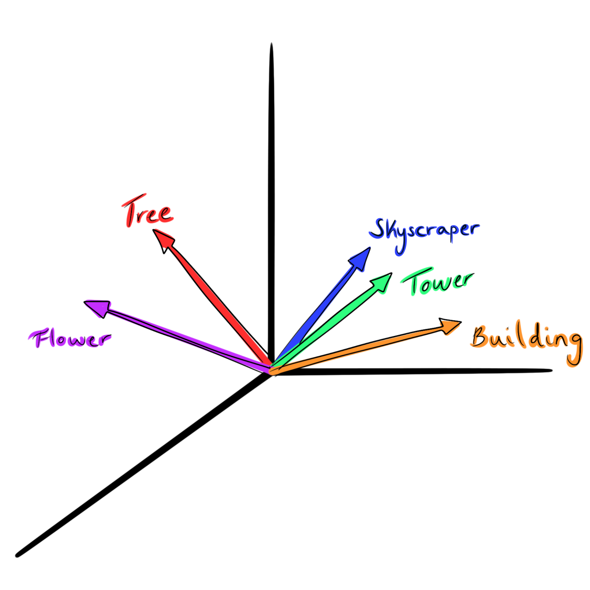
Fig. 6.2 Simple representation showing a few word vectors, where “building”, “tower”, and “skyscraper” are separate from “flower” and “tree”.#
The interesting thing about these vectors is that they add to each other. We can for example take the vector for “king”, subtract the vector for “man”, and add the vector for “woman”. The resulting vector will be very similar to the vector for “queen”.
Vectors code
This code allows you to play with vectors as described above. Some parts of this code will be unclear at this point, but we encourage you to come back to it after the python packages chapter and play around with it. By then you will also be able to install the gensim package locally and try this code for yourself in VS Code.
import gensim.downloader  # Import LLM library
import numpy as np  # Import numpy (more on this in later chapters)

model = gensim.downloader.load('glove-wiki-gigaword-50') # choose the model we will use from the gensim library


def cosine_similarity(a, b):
    '''
    Calculates the cosine similarity between two vectors "a" and "b"
    '''
    similarity = np.dot(a, b) / (np.linalg.norm(a) * np.linalg.norm(b))
    return similarity

# Define the vectors for the two terms we want to compare
term1 = model["queen"] # Get the vector for the word "queen"
term2 = model["king"] - model["man"] + model["woman"] # Calculate the vector for the 2nd term (king - man + woman)

print(cosine_similarity(term1, term2)) #Print the similarity between the two terms

# Try printing the terms independently: How many dimensions does the vector space have?
The output in the similarity between the two terms’s vectors given is 0.86095816, indicating a high similarity between them. If, however, we change the first term from “queen” to “dog”, the similarity value becomes 0.32295933, showing they are loosey related.
6.1.3.3. Attention and unembedding#
The input inserted into the LLM is thus a collection of embedded vectors, which when put together form a matrix. To get the output we are given, this matrix must then go through an attention and unembedding process which we will explain shortly.
Matrices
A matrix is just a way if representing various numbers put together in a rectangular grid arranged in rows and columns.
Matrix dimensions: The dimensions of a matrix refer to the shape of the grid, a matrix that has \((m)\) rows and \((n)\) columns is a 2 dimensional (2D) matrix, and is refered to as an \((m \times n)\) (read “m-by-n”) matrix.
1D matrices are also known as vectors.
A column vector is a matrix with m rows and one column \((m \times 1)\).
A row vector is a matrix with one row and n columns \((1 \times n)\).
An example of a way 2D matrices are used is in grayscale images. In a grayscale image matrix, each grid entry represents the intensity of its pixel.
A 3D matrix is a cube of numbers, which can be seen as, for example, a video-clip. We can see these clips as a 3D “matrix of matrices” with dimensions = (frames × image height × image width).
Why they matter: Matrices let us organise data compactly and perform operations like scaling, rotating, or combining information with simple arithmetic rules. Those same rules power everything from 3D graphics to neural-network layers.
We will go further into how matrices are commonly used in programming in the upcoming NumPy chapter.
6.1.3.3.1. Attention#
First this matrix will pass through an attention block. This attention block was a breakthrough in machine learning and is based on the paper: Attention Is All You Need.
How the attention block exactly works is beyond the scope of this course, but it has an important contribution as attention allows for the communication between vectors of the input. This is necessary as words can mean different things when used in different contexts. The word “bark”, for example, has a completely different meaning if it’s in the context of a dog or a tree. When using it in the sentence, its meaning must be determined from the context.
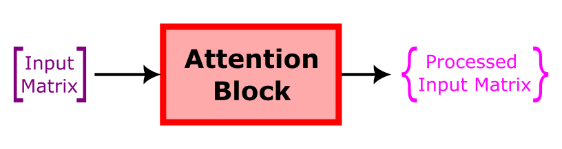
After the matrix has passed through the attention block and undergone the transformations within it, it will pass through a neural network, which we discussed earlier, and produce an output matrix.
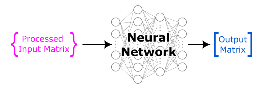
This output matrix will go through another attention block after which it will once again go through a neural network. These steps are repeated many times until the final matrix is obtained.
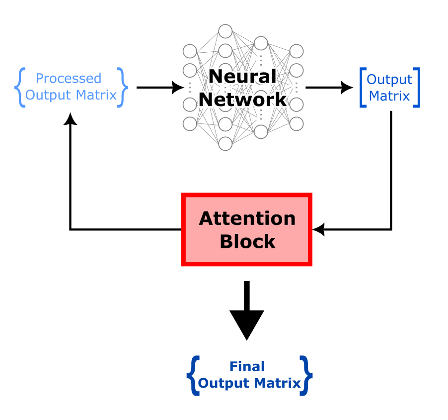
Fig. 6.3 Output matrix iteratively passed through the neural network and attention block until the final matrix is obtained.#
6.1.3.3.2. Unembedding#
When this process is finished, the final matrix needs to be unembedded. This simply means that a probability distribution is assigned to all possible tokens in the vocabulary of the network and, using these, the next word can be chosen as output.