13.2. Exercises#
For the exercises on this page, you will need to use NaNoPy package.
Each exercise carries the difficulty level indication:
[*] Easy
[**] Moderate
Exercise 13.2 ([*] Diagonal red line pixel by pixel)
Write a program that draws a diagonal red line by using the writer’s drawPixel function.
Exercise 13.3 ([*] Diagonal red line with drawLine)
Drawing lines pixel by pixel is not the most efficient way of doing so. Write a program that draws a
diagonal line using the writer’s drawLine function.
pen.drawLine (x1, y1, x2, y2, c)
The first two arguments (x1 and y1) indicate the origin of the line. The next two arguments (x2 and y2)
are the coordinates of the end of the line. The last argument (c) is the colour of the line.
Exercise 13.4 ([*] Changing colours)
The following code gives an error, try to ask AI to review and correct it for you. Then answer the following questions:
from NaNoPy import *

# Set up canvas
xSize = 400
ySize = 400
screen = canvas("Crossing Diagonals", xSize, ySize)
pen = writer(screen)

# Draw first diagonal: top-left to bottom-right (pink)
for i in range(min(xSize, ySize)):
    pen.drawPixel(i, i, color().pink)

# Draw second diagonal: top-right to bottom-left (orange)
for i in range(min(xSize, ySize)):
    pen.drawPixel(xSize - i - 1, i, color().orange)

# Update the display
screen.update()

# Keep the window open
screen.keepwindow()
Was AI able to correct it for you?
Now try and solve it yourself (Hint: the error mentions a problem with the “color” object, check the definition of
color()in the NaNoPy package).What was the issue? Why do you think AI might be unable to solve it for you?
Exercise 13.5 ([*] Random lines)
Write a program that draws several lines with random beginning and end points. Make sure each line starts and ends within the screen.
Hint: Make use of the random package in your code. Two examples are shown below:
import random as rnd

# Return random number between 0.0 and 1.0:
rnd.random()

# Return an integer between -2 and 2 (both included):
rnd.randint(-2,2)
Exercise 13.6 ([*] Blue circle)
Write a program that draws, centred on the screen, a blue circle with a radius of 50 pixels using the
writer’s drawCircle function:
pen.drawCircle (x, y, r, c, f)
The first two arguments (x and y) specify the centre of the circle. The third argument is the radius of
the circle. The fourth argument specifies the colour, and the last argument is a Boolean to specify
whether the circle should be filled or not.
Five seconds after drawing the circle, the screen should be cleared. The code below shows you how to how delay (pause in milliseconds) and then clear the screen:
screen.pause(5000)
screen.clear()
screen.update() # The screen needs to be updated to see the effect of the clearing
screen.keepwindow()
Exercise 13.7 ([*] Yellow flashing light)
Write a program that simulates a yellow flashing light in the middle of the graphical window that flashes until you stop the program.
Hint: use an infinite while loop (while screen.running(): . . . ), this will stop the program from running
when the window is closed. A while loop will perform its code as long as the condition you state is true.
Exercise 13.8 ([**] Moving particles)
Exercise A: Write a program, using the writer tool, that draws a red circle with a radius of 25 pixels at a random position on the graphical window. Each time you re-run the program, the position should be different (random). Make sure the circle always fits completely within the screen.
Exercise B:
Extend your code from exercise A such that it draws 100 red circles with radiuses of 5 pixels at random positions on the
graphical window. Your program should incorporate:
• Lists for the x and y coordinates.
• A loop to fill the list with random coordinates.
• A second loop to draw the circles.
Exercise C: Extend your code from exercise B such that it draws a 100 red circles. Every 100 ms a new circle should be added at a random position within the graphical window.
Exercise D: Extend your code from exercise C such that it draws 100 red circles one by one with 100 ms intervals at random positions on the graphical window, but now each time when a new circle is drawn, all previous circles should move one pixel down.
You can use a nested for loop: the outer loop determines the number of circles to be drawn and in the inner
loop those circles will be drawn.
Exercise 13.9 ([**] Simulation of moving objects)
In this exercise, you’ll be simulating the movement of objects through 2D space, such as a bouncing ball as well as random diffusion.
The code below simulates a ball moving from the left to the right side of the graphical window:
xSize = 800
ySize = 600
ballx = 1
bally = 300
dx = 1.0
nsteps = 1000

c = color().green

screen = canvas("title", xSize, ySize)
pen = writer(screen)

for i in range(nsteps):
    ballx = ballx + dx
    pen.drawCircle(ballx, bally, 5, c, True)
    screen.update()
    screen.pause(5)
    screen.clear()

screen.keepwindow()
Exercise A:
Run the code above and observe the result.
Then increase and decrease the speed at which the ball moves by modifying the value for dx.
Exercise B:
Extend the code such that the ball initially moves very fast, then gradually slows down before finally
stopping at the right border of the graphical window, by making dx depend on the position of the ball
within the graphical window.
Exercise C:
Extend the code such that the ball moves from top to bottom. Add a variable named dy.
Exercise D: Extend the code such that the ball moves in a diagonal line over the graphical window.
Exercise 13.10 ([**] Keeping an object within the screen)
In the previous exercise, you made the ball move over the screen, but the code was written in such a way that the ball moved from left to right, then stopped at the end of the graphical window. When simulating a less regulated movement of a ball, the path is less predictable or even unpredictable, so containing the ball inside the graphical window should be programmed in a different way.
Exercise A:
The algorithm for bouncing is very simple: when the ball reaches the top or bottom border of the
graphical window, change the sign of the displacement in vertical direction (dY = -dY). When the ball
bounces to the left or right side of the window, change the sign of the horizontal displacement (dX).
Write a Python program in which a ball moves in a diagonal line at constant speed and bounces when it reaches one of the borders of the graphical window. The ball should keep moving until the graphical window is closed. Try different angles of movement.
Exercise B:
Extend your code from exercise A such that it simulates the bouncing of a ball in the
presence of gravity: decrease the ball displacement in the vertical direction when the ball is moving
upwards, and increase the ball displacement in the vertical direction when the ball is moving
downwards by subtracting a small value from dY (e.g., dY = dY - 0.1).
If the ball bounces higher each step, adjust the program so that the peaks are lower each time the
ball bounces.
Exercise 13.11 ([**] Random particle diffusion)
In this exercise, you will simulate the random movement of a particle.
Exercise A:
Generate random values for dX and dY between, for instance, -5 and 5. The particle should not be
allowed to move outside the graphical window. You can change the speed at which the particle moves
by varying the range of your random values.
Exercise B: Extend your code such that instead of one particle,your program works with 100 particles and makes them move randomly.
Hints:
You’ll need a list with the
xcoordinates for the particles, and a list with theycoordinates for the particles.Perform separate tasks in separate loops.
When you update your graphical window for every particle individually, your program will slow down. To avoid this, first change the coordinates of all particles and draw them to the graphical window before updating it.
Exercise 13.12 ([**] Particle collision)
Exercise A: Write a program where two different types of particles diffuse randomly within the graphical window. Use ten particles of each type, where each type has its own colour, size, and speed.
Hint: Store the properties of each particle in a list. Because the properties are different types of variables, create a list for each property. For instance, one list to store the sizes of all 20 particles, another list to store the colors of all the 20 particles, etc.
Exercise B:
Extend your code such that the particles seize to move when they meet/collide with a particle of the other type. We define meeting/collision as the distance of less than 15 coordinate units. Use the following equation of Pythagoras to calculate the distance d between two particles P and Q:
\(d = \sqrt{(Px - Qx)^2 + (Py - Qy)^2}\)
Hints:
In case it takes too long before particles stop, increase the distance for collision.
In exercise A, you’ve created multiple lists in which you store the different properties of each particle. In that exercise it might seem convenient to create a different lists per particle type, but would that still be convenient if you had, e.g., 300 different types of particles, all interacting with each other? Instead, try to see the type of a particle as a “property” of being of a different type. So, you can create a list in which you store the type of each particle (particle type list), a list to store the sizes of all the particles (particle size list), a list to store the shapes of all the particles (particle shape list), a list to store colours (particle colour list), etc.
Exercise C: Extend your code such that it only stops particles from moving when they meet a particle of the other type that is moving as well (with a distance less than 5 coordinate units). Increase the number of particles and change the ratio between the two types to 40:60.
Hint: use an extra list in which you store the property of whether a particle is moving.
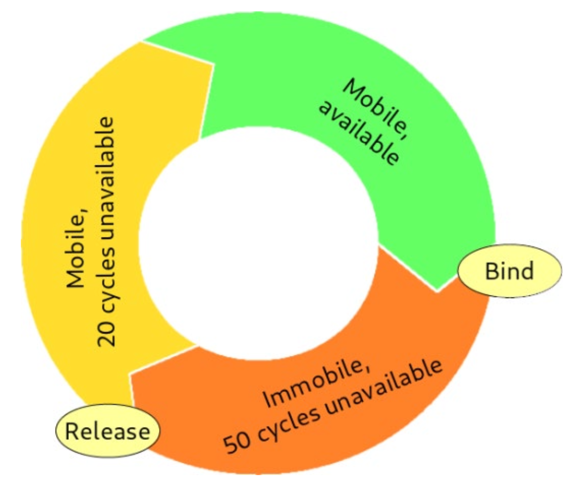
Exercise D: Extend your program such that if a particle binds (meets) a particle of the other type, it should change colour, stop moving, and stay bound for 50 timesteps. After those 50 timesteps, the particles should again change colour and start moving again, but remain unable to bind again for another 20 timesteps. After those 20 timesteps, the particles should go back to their original color and be able to bind again.
Hint: Create an extra variable (list) containing a property of the particle keeping track of the passed
runs of the while loop. This will help to keep track of the timesteps in which the particle is bound or unable to
bind.
Exercise E: Extend your code such that it lets particles bind with a probability of 0.1 per timestep and release with a probability of 0.01 per timestep. Notice that you will need to know which particles are bound together to release them both at the same time step.
Hint: Use random function to create a probability to test.
Exercise 13.13 ([**] Escape the container and monitor the situation)
Exercise A: In this exercise, you will build upon your code from Random particle diffusion, Exercise B. There, you were able to keep the particles inside the graphical window. In this exercise, you’re asked to adjust the borders in such a way that 100 particles are now contained in a specified area. This container should be smaller than the screen. Make 3 versions with a square, a rectangular, and finally with a round container.
Hint: testing whether a particle is inside a square or rectangular container is similar to testing if it stays within the screen, like you did before. However, testing whether a particle is inside a circle is a bit different. A circle is made up of a sine and a cosine function, centred on the middle and is as big as its radius. If the distance between a particle and the centre of a circle is larger than the radius of that circle, the particle is not inside the circle anymore. Use this information to think of a test to keep the particles within the round container.
Exercise B: Extend your program from exercise A such that instead of a single round container you make three round containers and let there be 100 moving particles in each container. The particles should not escape the containers.
Hint: the particles should get a location within one of the three containers before starting the simulation. All particles should be tested for all containers even if they are not inside that particular container. If a displacement leads to the future location of a particle outside of any container, this displacement should not be made.
Exercise C: In exercise B we tested if particles were inside any of three containers. The code to check if particles are inside a container is very similar for each container, with just some changes in the location of the container and the size of the container. When there are many similar sections of code, you will recall from a previous book section that it’s useful to define a Python function.
In this exercise, you’re asked to rewrite the code to check if a particle is in a container using a function. The inputs should be the X and Y location of the particle, and the X and Y location and radius of a container. The output should
be a Boolean returning True if the particle is in the container and False if it is outside. For example,
def incircle(x, y, x_container, y_container, r_container):
    output = # code to test if x and y are inside container
    return output
Now you can check if a particle is inside the container using:
if incircle(x,y,x_c,y_c,r):
    # code to do if particle is in the container
Exercise D: Extend your program from exercise A, use the round container and the function from exercise C. When a particle tries to escape the container, introduce a chance of 25 % that it will succeed. See what happens when you vary the chance.
Hint: Use the random function to create a probability.
Exercise E: Extend your code from exercise D such that if a particle escapes the container, make it change colour and size.
Exercise F: Extend your program from exercise E such that you keep track of the number of particles inside and outside of the container. Plot these numbers against time in a graph in a new graphical window positioned next to the graphical window with the moving particles. Therefore, another screen is required. Define this directly after the original screen:
chart = canvas("charttitle", xSize, ySize, xpos=50, ypos=50)
The last two arguments define the location of the chart, in this case at 50 pixels outside of the left upper corner of your screen.
Hint: Think about how you would draw a dynamic graph using the NaNoPy package and what type of graph you want to plot.