Algebraic Distance in Geometrical Optics

There exists a method to deal with the sign convention in geometrical optics which uses so-called algebraic distances. It is a matter of taste but this method which is mostly taught in France may be an interesting alternative to the convention used in Chapter 2.

Definition

Let there be two points A and B in an affine space through which passes a directed line (a line with a direction, i.e. generated by a nonzero vector \(\vec{v}\)). We introduce the algebraic distance \(\overline{AB}\) from A to B to be the real number such that :

1. its absolute value is the distance between A and B

2. if the value is non-zero:

3. \(\overline{AB}\) is positive in the case the vector \(\overrightarrow{\rm AB}\) has the same direction as \(\vec{v}\), i.e. \(\overrightarrow{\rm AB}= k\vec{v}\) with \(k>0\);

4. \(\overline{AB}\) is negative otherwise.

It follows that

\[\begin{align*} \overline{AB}=\dfrac{\overrightarrow{\rm AB}\cdot\vec{v}}{\Vert\vec{v}\Vert} \end{align*}\]

Note that to define the algebraic distance, no choice for the origin is needed, only a vector that defines the direction of the line.

Properties

The algebraic distance has the following properties:

• \(\overline{AA}=0\),

• \(\overline{AB}=-\overline{BA}\),

• for three points A, B and C all on the same line:

\[\begin{align*} \overline{AC}=\overline{AB}+\overline{BC} \end{align*}\]

irrespective of the position of B relative to A and C on the line.

The last point can can be shown using the analogous equality for vectors:

\[\begin{align*} \overrightarrow{\rm AC}= \overrightarrow{\rm AB}+\overrightarrow{\rm BC} \end{align*}\]

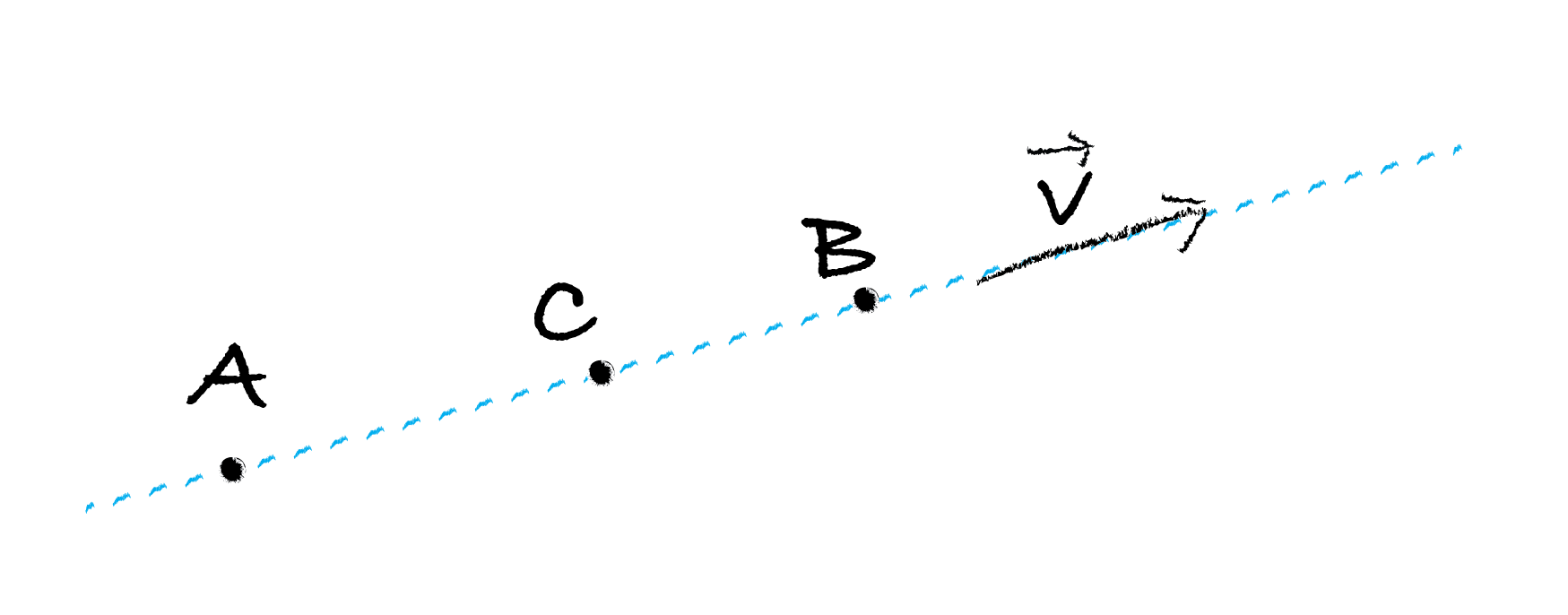
Fig. 136 Definition the different points in an optical system.

Algebraic distance in Optics

When we use the algebraic distance in optics, we use the following conventions:

1. Light propagates from left to right;

2. The optical axis is positively oriented towards the right (i.e. in the direction the light propagates);

3. the vertical axis, perpendicular to the optical axis is positively oriented upwards.

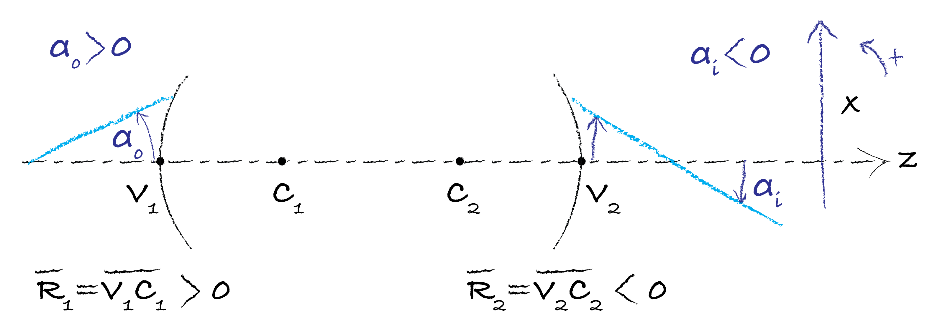
Fig. 137 Definition the different points in an optical system.

In Fig. 137, the definition of positive ray angle and positive radii of curvature are defined:

\[\begin{align*} \overline{R_1}\equiv\overline{V_1C_1}>0, \mbox { and } \overline{R_2}=\overline{V_2C_2}<0. \end{align*}\]

One Spherical Surface

Let us consider a spherical interface between two media with different index of refraction \(n_1\) and \(n_2\) as shown in Fig. 138. Let C be the center of the sphere and let V be the vertex, i.e. the point of intersection of the sphere and the optical axis. One can show that for the image point \(A_2\) of point \(A_1\):

(517)\[ \dfrac{n_2}{\overline{VA_2}}-\dfrac{n_1}{\overline{VA_1}}=\dfrac{n_2-n_1}{\overline{VC}}=V, \]

and that the transverse magnification can be written as:

\[\begin{align*} M=\dfrac{\overline{VA_2}}{n_2}.\dfrac{n_1}{\overline{VA_1}}. \end{align*}\]

If the object is at infinity \(A_2=F_2\) is the image focal point and

\[\begin{align*} \dfrac{n_2}{\overline{VF_2}}=\dfrac{n_2-n_1}{\overline{VC}}=P, \end{align*}\]

where \(P\) is the power of the surface. If the image is at the infinity, \(A_1=F_1\) is the object focal point and

\[\begin{align*} \dfrac{n_1}{\overline{VF_1}}=-\dfrac{n_2-n_1}{\overline{VC}}=-P \end{align*}\]

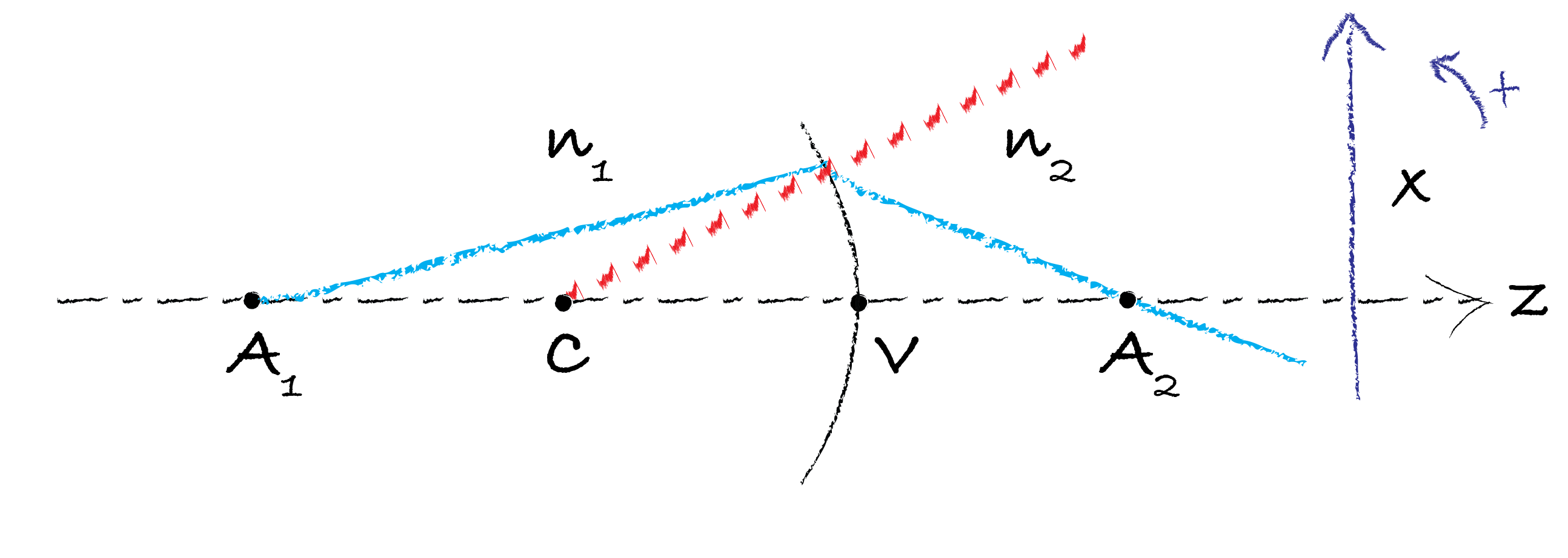
Fig. 138 Spherical surface separating two different media.

When the interface is flat: \(\overline{VC}\rightarrow \infty\), we get

\[\begin{align*} \dfrac{n_2}{\overline{VA_2}}=\dfrac{n_1}{\overline{VA_1}} \end{align*}\]

We can easily rewrite the Eq. (517) as function of the center instead of the summit by exchanging V with C and \(n_1\) with \(n_2\):

\[\begin{align*} \dfrac{n_1}{\overline{CA_2}}-\dfrac{n_2}{\overline{CA_1}}=\dfrac{n_1-n_2}{\overline{CV}} \end{align*}\]

and for the transverse magnification:

\[\begin{align*} M=\dfrac{\overline{CA_2}}{\overline{CA_1}} \end{align*}\]

The last relation is usually called the relation of Descartes and put in relation \(F_1\) and \(F_2\) with the vertex:

(518)\[\begin{align*} \frac{\overline {VF_2}}{\overline {VA_2}}+{\frac {\overline {VF_1}}{\overline {VA_1}}}=1 \end{align*}\]

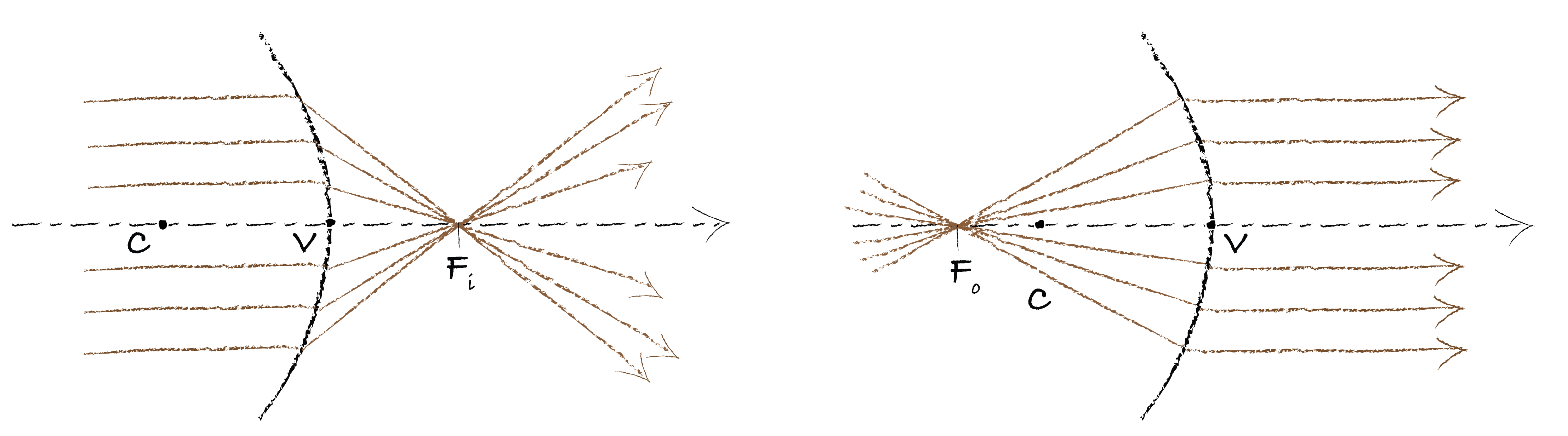
Fig. 139 Dioptre sph’{e]}rique: position of the image focal point and the object focal point

The relation of Newton is an other way to link the position of the object and the one of the image via the focal points:

\[\begin{align*} \overline{F_2A_2} \cdot \overline{F_1A_1} = \overline{VF_2} \cdot \overline{VF_1} \end{align*}\]

Mirror

For the mirror, we define \(V\) as the vertex (the meeting point between the mirror and the optical axis), \(C\) the center of the curvature and \(F\) the focal point as show in Fig. 140. For a concave mirror \(\overline{VC}=2\overline{VF}<0\) and for the convex mirror, \(\overline{VC}=2\overline{VF}>0\).

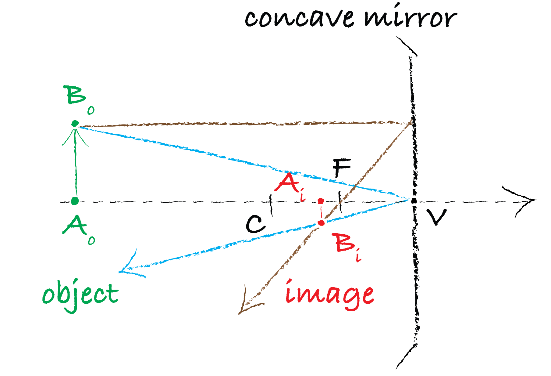
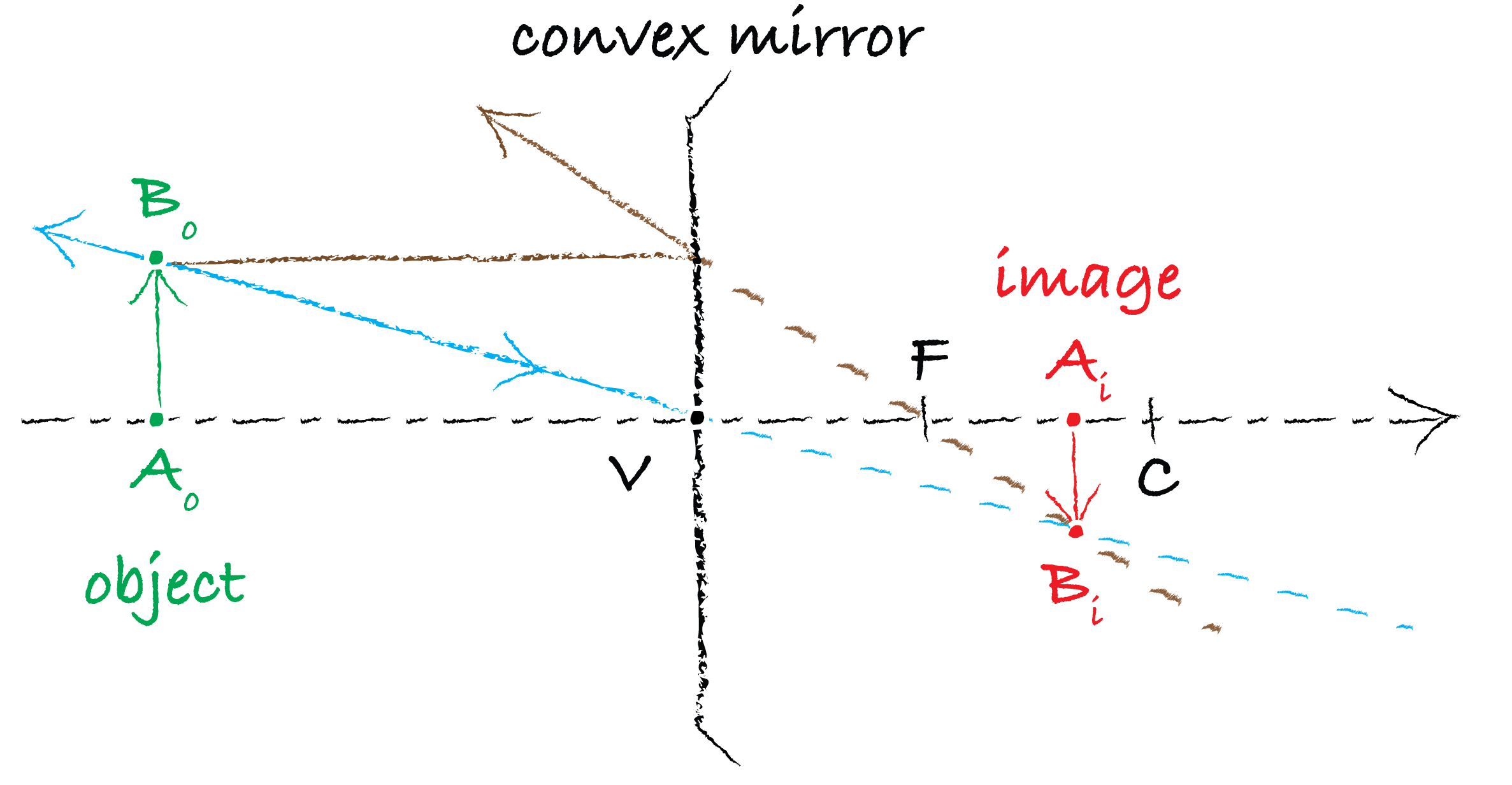
Fig. 140 Definition of \(O\), \(F_o\) and \(F_i\) for a concave (left) and a convex (right) mirror.

If a point A is placed on the right of the mirror, i.e. \(\overline{VA}>0\), the point is consider virtual. Be aware that if you look at the mirror yourself, you will be able to “image” this virtual point. To convince yourself, just use a spoon.

We can derive the law of conjugation the works for any spherical mirror independent on its curvature:

\[\begin{align*} \dfrac{1}{\overline{VA_i}}+\dfrac{1}{\overline{VA_o}}=\dfrac{2}{\overline{VC}} \end{align*}\]

The magnification can also be derived:

\[\begin{split}\begin{align*} M&\equiv\dfrac{\overline{A_iB_i}}{\overline{A_oB_o}}\\ &=\dfrac{\overline{FV}}{\overline{FA_o}}=\dfrac{\overline{FA_i}}{\overline{FV}}=-\dfrac{\overline{VA_i}}{\overline{VA_o}} \end{align*}\end{split}\]

As we have done earlier, we can rewrite these equations with center instead of the summit:

\[\begin{align*} \dfrac{1}{\overline{CA_i}}+\dfrac{1}{\overline{CA_o}}=\dfrac{2}{\overline{CV}} \end{align*}\]

The magnification can also be derived with C as origin:

\[\begin{split}\begin{align*} M&\equiv\dfrac{\overline{A_iB_i}}{\overline{A_oB_o}}\\ &=\dfrac{\overline{CA_i}}{\overline{CA_o}} \end{align*}\end{split}\]

Spherical lens

Spherical lenses are made of glass and are bounded by two spherical surfaces of curvature \(\overline{R_1} = \overline{C_1V_1}\) and \(\overline{R_2} = \overline{C_2V_2}\), with centres \(C_1\) and \(C_2\) and vertices \(V_1\) and \(V_2\) respectively. When \(\overline{R_1}>0\) and \(\overline{R_2}<0\), the lens is biconvex; when \(\overline{R_2}>0\) and \(\overline{R_1}<0\) it is biconcave. They are thin when the distance (\(V_1V_2\)) is very small compared to the radii of curvature \(R_1\) and \(R_2\).

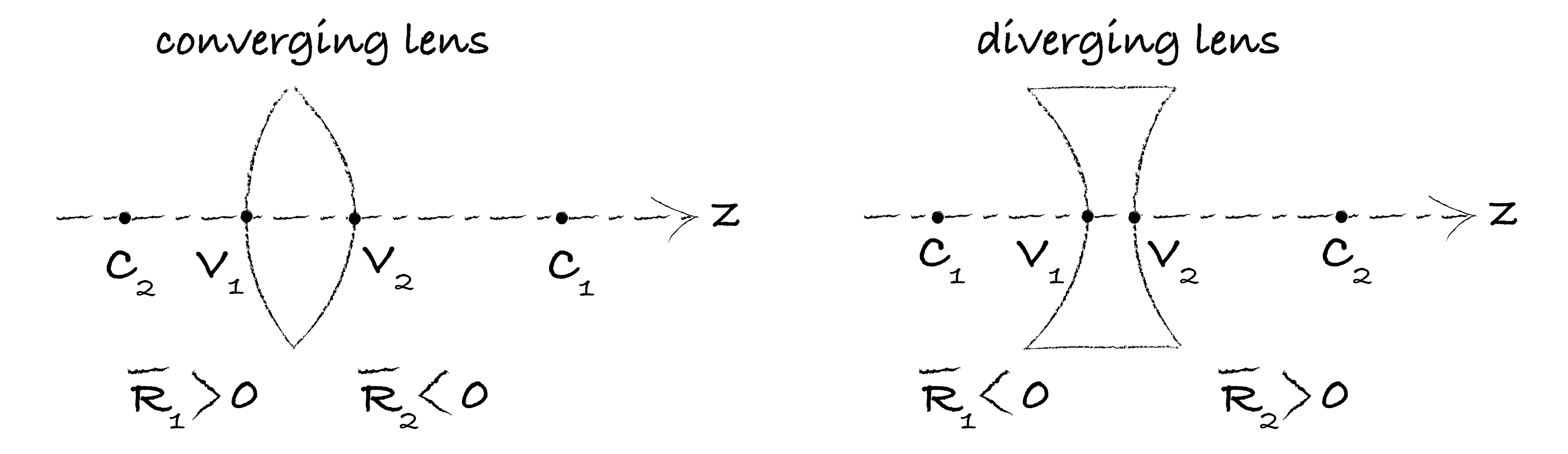
Fig. 141 Converging and diverging lens depending on the curvatures.

Thin spherical lens

When considering a thin spherical lens, we define 3 points \(O\), \(F_o\) and \(F_i\), respectively the center of the lens, the focal object point and focal image point. As shown in Fig. 142, we can say:

• $F_o$ is the point from which all rays hand up parallel to the optical axis when exiting the lens are originating;\

• \(F_i\) is the point were all the rays parallel to the optical axis coming towards the lens converges to.

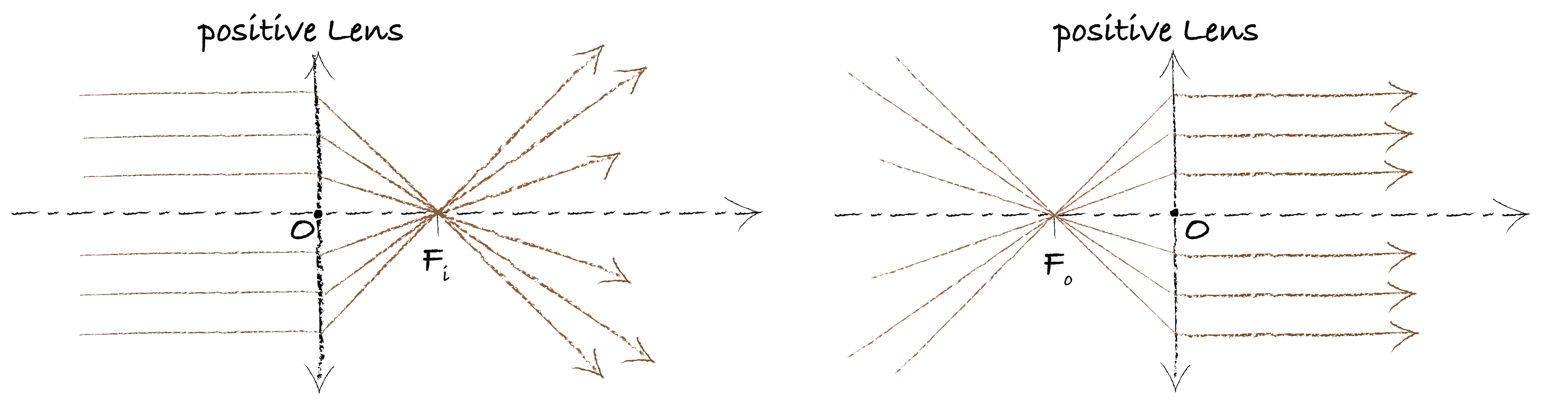
Fig. 142 Definition of \(O\), \(F_o\) and \(F_i\) for a positive lens.

The image focal length \(f_i\) of a lens is defined as the algebraic quantity :

\[\begin{align*} f_i\equiv\overline{OF_i}=-\overline{OF_o}=f_o \end{align*}\]

while we also introduce the object focal length \(f_o\).

• In the case of a positive lens, the image focal distance \(f_i\) is positive, i.e. \(\overline{OF_i}>0\) and \(\overline{OF_o}<0\).

• In the case of a negative lens, the image focal distance \(f_i\) is negative, i.e. \(\overline{OF_i}>0\)

The algebraic quantity called the diopter \(\cal{D}\) of a thin lens is:

\[\begin{align*} \cal{D}&\equiv\dfrac{1}{\overline{OF_i}}=(1-n)\left(\dfrac{1}{\overline{V_2C_2}}-\dfrac{1}{\overline{V_1C_1}}\right) \end{align*}\]

where \(n\) is the index of refraction of the glass.

For any lens system defined with \(F_i\) as the image focal point, we now only have one equation which is always valid:

\[\begin{align*} \dfrac{1}{\overline{OF_i}}=\dfrac{1}{\overline{OA_i}}-\dfrac{1}{\overline{OA_o}} \end{align*}\]

where the point \(A_i\) is image of the point \(A_o\) through the lens. Notice that we do not need to know where \(A_o\) is with regards to the lens to write the formula nor if we deal with a positive lens. If in your calculation you find for example that \(\overline{OA_i}<0\) then you know that the image is virtual.

We can also define the magnification as:

\[\begin{align*} M\equiv\dfrac{\overline{A_iB_i}}{\overline{A_oB_o}}=\dfrac{\overline{OA_i}}{\overline{OA_o}} \end{align*}\]

where the point \(B_i\) is the image of the object point \(B_o\). The sign of \(M\) will automatically give you if the image is inverted or not.

Fig. 143 shows the case where the image is inverted compare to the object where \(\overline{OA_i}\) is positive and \(\overline{OA_o}\) is negative.

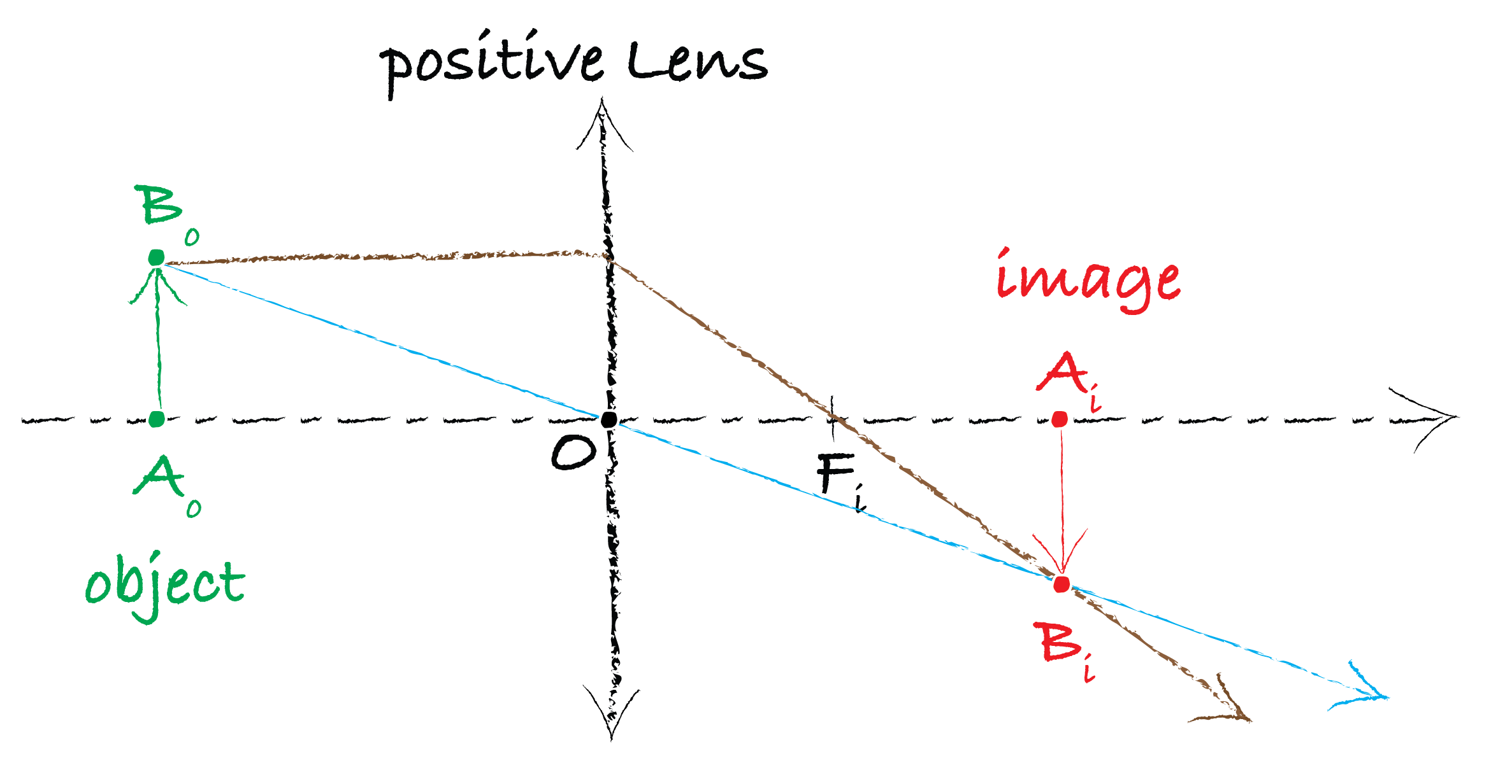
Fig. 143 Image of an object from a positive lens.