Interference and Coherence

What you should know and be able to do after studying this chapter

• Understand time coherence and spatial coherence.

• Know how the degree of time coherence can be measured with a Michelson interferometer.

• Understand the connection between the time coherence and the frequency bandwidth.

• Know that the spatial coherence of the field in two points in space can be measured with Young’s two-slit experiment.

• Understand that spatial coherence increases by propagation.

• Understand how the size of an incoherent source such as a star can be derived from measuring the spatial coherence at large distance from the source.

• Know the definition of fringe contrast.

• Know and understand the three Laws of Fresnel-Arago.

Introduction

Although the model of geometrical optics helps us to design optical systems and explains many phenomena, there are properties of light that require a more elaborate model. For example, interference fringes observed in Young’s double-slit experiment or the Arago spot (Fig. 70) indicate that light is more accurately modelled as a wave.

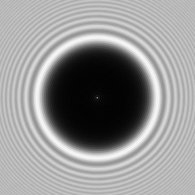
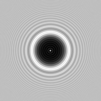
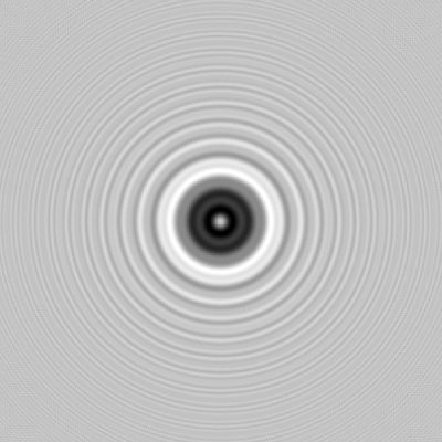
Fig. 70 The Arago spot is the bright spot which occurs at the centre of the shadow of a circular disc and which is caused by diffraction. The disc has diameter 4 mm, 2 mm and 1 mm, from left to right, the wavelength is 633 nm and the intensity is recorded at 1 m behind the disc and has width of 16 mm

In this chapter we will study the wave model of light. It will be shown that the extent to which light can show interference depends on a property called coherence. In the largest part of the discussion we will assume that all light has the same polarisation, so that we can treat the fields as scalar. In the last section we will look at how polarisation affects interference, as described by the Fresnel-Arago laws.

It is important to note that the concepts of interference and coherence are not just restricted to optics. Since quantum mechanics dictates that particles have a wave-like nature, interference and coherence also play a role in e.g. solid state physics and quantum information.

External sources in recommended order

• KhanAcademy - Interference of light waves: Playlist on wave interference at secondary school level.

• Yale Courses - 18. Wave Theory of Light

Interference of Monochromatic Fields of the Same Frequency

Let us first recall the basic concepts of interference. What causes interference is the fact that light is a wave, which means that it not only has an amplitude but also a phase. Suppose for example we evaluate a time-harmonic field in two points

\[\begin{align*} \mathcal{U}_1(t)=\cos(\omega t), \quad \mathcal{U}_2(t)=\cos(\omega t +\varphi). \end{align*}\]

Here \(\varphi\) denotes the phase difference between the fields at the two points. If \(\varphi=0\), or \(\varphi\) is a multiple of \(2\pi\), the fields are in phase, and when they are added they interfere constructively

\[\begin{align*} \mathcal{U}_1(t)+\mathcal{U}_2(t)=\cos(\omega t) + \cos(\omega t + 2 m \pi) =2\cos(\omega t). \end{align*}\]

However, when \(\varphi=\pi\), or more generally \(\varphi=\pi+ 2 m \pi\), for some integer \(m\), then the waves are out of phase, and when they are superimposed, they interfere destructively.

\[\begin{align*} \begin{split} \mathcal{U}_1(t)+\mathcal{U}_2(t)&=\cos(\omega t)+\cos(\omega t+\pi+ 2 m\pi) &=\cos(\omega t)-\cos(\omega t) &=0. \end{split} \end{align*}\]

We can sum the two fields for arbitrary \(\varphi\) more conveniently using complex notation:

\[\begin{align*} \mathcal{U}_1(t)=\text{Re}[ e^{-i\omega t}], \; \; \mathcal{U}_2(t) =\text{Re}[ e^{-i\omega t}e^{-i\varphi}]. \end{align*}\]

Adding gives

(294)\[\begin{align*} \mathcal{U}_1(t)+\mathcal{U}_2(t)&= \text{Re}[e^{-i\omega t}(1+e^{-i\varphi})] &=\text{Re}[e^{-i\omega t}e^{-i\varphi/2}(e^{i\varphi/2}+e^{-i\varphi/2})] &=\text{Re}[e^{-i\omega t}e^{-i\varphi/2}2\cos(\varphi/2)] &= 2\cos(\varphi/2)\cos(\omega t+\varphi/2). \end{align*}\]

For \(\varphi= 2 m \pi\) and \(\varphi=\pi+2 m \pi\) we retrieve the results obtained before. It is important to realize that what we see or detect physically (the ‘brightness’ of light) does not correspond to the quantities \(\mathcal{U}_1\), \(\mathcal{U}_2\). After all, \(\mathcal{U}_1\) and \(\mathcal{U}_2\) can attain negative values, while there is no such thing as ‘negative brightness’. What \(\mathcal{U}_1\) and \(\mathcal{U}_2\) describe are the fields, which may be positive or negative. The ‘brightness’ or the irradiance or intensity is given by taking an average over a long time of \(\mathcal{U}(t)^2\) (see (83)), we shall omit the factor \(\sqrt{\epsilon/\mu_0}\)). As explained in Chapter 1, we see and measure only the long time-average of \(\mathcal{U}(t)^2\), because at optical frequencies \(\mathcal{U}(t)^2\) fluctuates very rapidly. We recall the definition of the time average over an interval of length \(T\) at a specific time \(t\) given in (88) in Chapter 1:

(295)\[\begin{align*} \braket{f(t)}= \frac{1}{T}\int_{t}^{t+T}f(t')\,\text{d}t', \end{align*}\]

where \(T\) is a time interval that is the response time of a typical detector, i.e. \(T\approx 10^{-6}\,\text{s}\) which is extremely long compared to the period of visible light which is of the order of \(10^{-14}\, \text{s}\). For a time-harmonic function, the long-time average is equal to the average over one period of the field and hence it is independent of the time \(t\) at which it is taken. Indeed for (294) we get

\[\begin{split}\begin{align*} I &= \braket{(\mathcal{U}_1(t)+\mathcal{U}_2(t))^2} &=4\cos^2(\varphi/2) \braket{\cos^2(\omega t+\varphi/2)} &= 2(1+\cos\phi) \braket{\cos^2(\omega t+\varphi/2)} \\ &= 1 +\cos(\varphi) \end{align*}\end{split}\]

Using complex notation one can obtain this result more easily. Let

\[\begin{align*} \mathcal{U}_1(t)=\text{Re}[U_1 e^{-i\omega t}], \quad \mathcal{U}_2(t)=\text{Re}[U_2 e^{-i\omega t}], \end{align*}\]

where

\[\begin{align*} U_1=1, \quad U_2=e^{-i\varphi}. \end{align*}\]

Then we find

\[\begin{align*} \begin{split} |U_1+U_2|^2&=|1+e^{-i\varphi}|^2 &=(1+e^{i\varphi})(1+e^{-i\varphi}) &=1+1+e^{-i\varphi}+e^{i\varphi} &=2+2\cos(\varphi), \end{split} \end{align*}\]

hence

(296)\[\begin{align*} I = \frac{1}{2}|U_1 + U_2|^2. \end{align*}\]

To see why this works, recall Eq. (89) and choose \(A=B=U_1+U_2\).

Remark. To shorten the formulae, we will omit in this chapter the factor \(1/2\) in front of the time-averaged intensity.

Hence we define \(I_1=|U_1|^2\) and \(I_2=|U_2|^2\), and we then find for the time-averaged intensity of the sum of \(U_1\) and \(U_2\):

(297)\[\begin{split}\begin{align*} I &= |U_1+U_2|^2=(U_1+U_2)(U_1+U_2)^* \\ &= |U_1|^2+|U_2|^2+U_1U_2^*+U_1^* U_2 \\ &= I_1+I_2+2\text{Re}[ U_1 U_2^* ] \\ &= I_1 + I_2 + 2 \sqrt{I_1}\sqrt{I_2}\cos(\phi_1-\phi_2), \end{align*}\end{split}\]

where \(\phi_1\) and \(\phi_2\) are the arguments of \(U_1\) and \(U_2\) and \(\phi_1-\phi_2\) is the phase difference. The term \(2\text{Re}[U_1^* U_2]\) is known as the interference term. In the famous double-slit experiment (which we will discuss in a later section), we can interpret the terms as follows: let us say \(U_1\) is the field that comes from slit 1, and \(U_2\) comes from slit 2. If only slit 1 is open, we measure on the screen intensity \(I_1\), and if only slit 2 is open, we measure \(I_2\). If both slits are open, we would not measure \(I_1+I_2\), but we would observe fringes due to the interference term \(2\text{Re}[U_1^* U_2]\).

The intensity (297) varies when the phase difference varies. These variations are called fringes. The fringe contrast is defined by

(298)\[\begin{align*} \textrm{ Fringe contrast} = \frac{ I_{max}-I_{min}}{I_{max}+I_{min}}. \end{align*}\]

It is maximum and equal to \(1\) when the intensities of the interfering fields are the same. If these intensities are different the fringe contrast is less than 1.

More generally, the intensity of a sum of multiple time-harmonic fields \(U_j\) all having the same frequency is given by the coherent sum

\[\begin{align*} I=\left|\sum_j U_j\right|^2. \end{align*}\]

However, we will see in the next section that sometimes the fields are unable to interfere. In that case all the interference terms of the coherent sum vanish, and the intensity is given by the incoherent sum

\[\begin{align*} I=\sum_j |U_j|^2. \end{align*}\]

Coherence

In the discussion so far we have only considered monochromatic light, which means that the spectrum of the light consists of only one frequency. Although light from a laser often has a very narrow band of frequencies and therefore can be considered to be monochromatic, purely monochromatic light does not exist. One reason that light can not be perfectly monochromatic is that any source must have been switched on a finite time ago. Hence, all light consists of multiple frequencies and therefore is polychromatic. Classical light sources such as incandescent lamps and also LEDs have relatively broad frequency bands. The question then arises how differently polychromatic light behaves compared to the idealised case of monochromatic light. To answer this question, we must study the topic of coherence. One distinguishes between two extremes: fully coherent and fully incoherent light, while the degree of coherence of practical light is somewhere in between. Generally speaking, the broader the frequency band of the source, the more incoherent the light is. It is a very important observation that no light is actually completely coherent or completely incoherent. All light is partially coherent, but some light is more coherent than others.

An intuitive way to think about these concepts is in terms of the ability to form interference fringes. For example, with laser light, which usually is almost monochromatic and hence coherent, one can form an interference pattern with clear maxima and minima in intensities using a double slit, while with sunlight (which is incoherent) this is much more difficult. Every frequency in the spectrum of sunlight gives its own interference pattern with its own frequency dependent fringe pattern. These fringe patterns wash out due to superposition and the total intensity therefore shows little fringe contrast, i.e. the coherence is less. However, it is not impossible to create interference fringes with natural light.^[1] The trick is to let the two slits be so close together (of the order of \(0.02 \, \text{mm}\)) that the difference in distances from the slits to the sun is so small for the fields in the slits to be sufficiently coherent to interfere. To understand the effect of polychromatic light, it is essential to understand that the degree to which the fields in two points are coherent, i.e. the ability to form fringes, is determined by the difference in distances between these points and the source. The distance itself to the source is not relevant. This will be made clear in this chapter.

Coherence of Light Sources

In a conventional light source such as a gas discharge lamp, photons are generated by spontaneous emission with energy equal to the energy difference between certain electronic states of the atoms of the gas. These transitions have a duration of the order of \(10^{-8}\) to \(10^{-9} \, \text{s}\). Because the emitted wave trains are finite, the emitted light does not have a single frequency; instead, there is a band of frequencies around a centre frequency with width roughly equal to the reciprocal of the duration of the wave train. This spread of frequencies is called the natural linewidth. Random thermal motions of the molecules cause further broadening due to the Doppler effect. In addition, the atoms undergo collisions that interrupt the wave trains and therefore further broaden the frequency spectrum.

We first consider a single emitting atom. When collisions are the dominant broadening effect and these collisions are sufficiently brief, so that any radiation emitted during the collision can be ignored, an accurate model for the emitted wave is a steady monochromatic wave train at frequency \(\mathbf{a}r{\omega}\) at the centre of the frequency band, interrupted by random phase jumps each time that a collision occurs. The discontinuities in the phase due to the collisions cause a spread of frequencies around the centre frequency. An example is shown in Fig. 71. The average time \(\tau_0\) between the collisions is typically less than \(10^{-10}\) s which implies that on average between two collisions roughly \(10^6\) harmonic oscillations occur and that during an atom transition of the order of hundred collisions may occur. The coherence time \(\Delta \tau_c\) is defined as the maximum time interval over which the phase of the electric field can be predicted. In the case of collisions-dominated emission by a single atom, the coherence time is equal to the average time between subsequent collisions: \(\Delta \tau_c = \tau_0\text{ }10^{-10}\) s.

To understand coherence and incoherence, it is helpful to use this model for the emission by a single atom as harmonic wave trains of many thousands of periods interrupted by roughly hundred random phase jumps. Due to the random phase jumps, the interference term of the sum of harmonic wave trains emitted by two atoms when integrated of the relatively long integration time of a detector becomes a sum over integrals over time intervals of average length \(\tau_0\):

\[ \sum_{j} \int_0^{\tau_0} \cos(\omega t) \cos(\omega t + \phi_j) \text{d} t,\]

where the sum is over roughly one hundred random phase jumps during the total duration of the wave trains. The random phase jumps lead to cancellation of the integrals and hence the interference term vanishes. We conclude that over the integration time of typical detectors

Note

Light trains which have been spontaneously emitted by different atoms can not interfere.

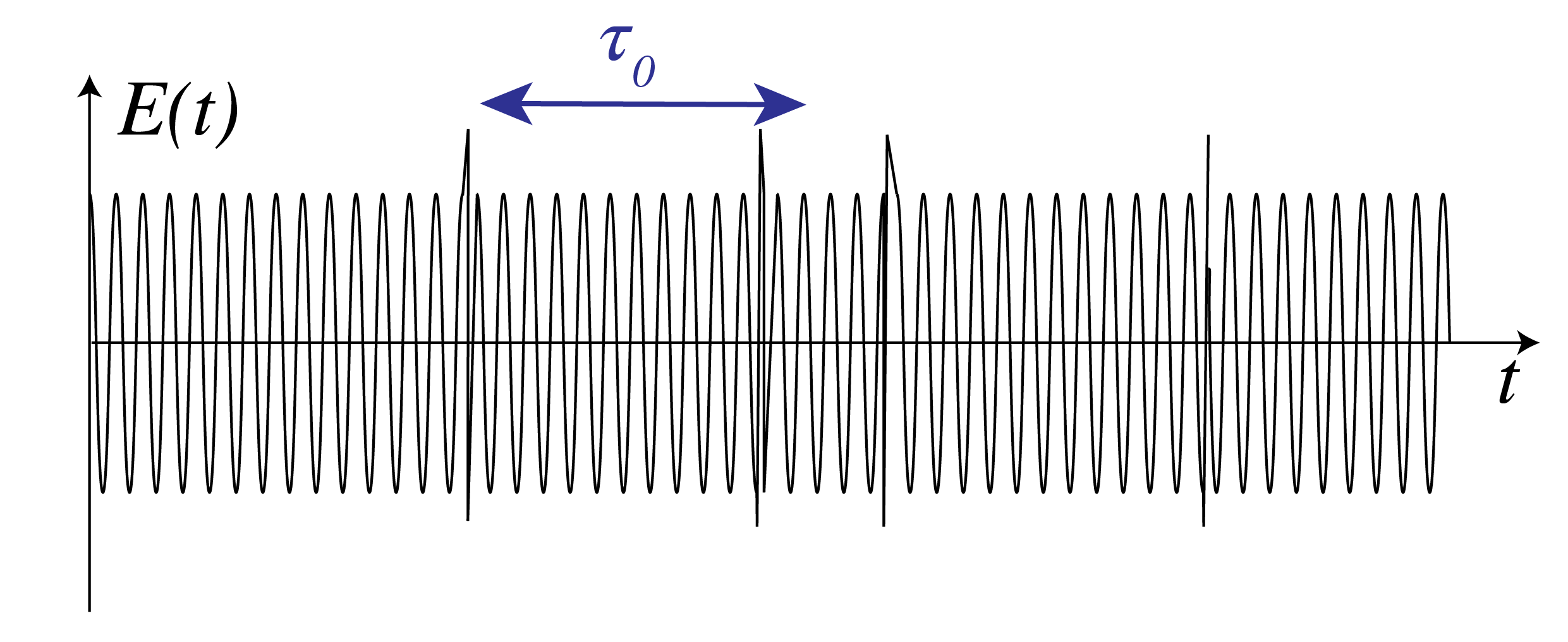
Fig. 71 The electric field amplitude of the harmonic wave train radiated by a single atom at the centre frequency \(\mathbf{a}r{\omega}\). The vertical lines are collisions separated by periods of free flight with mean duration \(\tau_0\). The quantity \(\mathbf{a}r{\omega}\tau_0\), which is the number of periods in a typical wave train, is chosen unrealistically small (namely 60, whereas a realistic value would be \(10^5\)) to show the random phase changes.

The coherence time and the width \(\Delta \omega\) of the frequency line are related as

(299)\[\begin{align*} \Delta \tau_c = \frac{2\pi}{\Delta \omega}. \end{align*}\]

The coherence length is defined by

(300)\[\begin{align*} \Delta \ell_{c}= c \Delta \tau_c. \end{align*}\]

Since \(\lambda \omega = 2\pi c\), we have

(301)\[\begin{align*} \frac{\Delta \lambda}{\mathbf{a}r{\lambda}} = \frac{\Delta \omega}{\mathbf{a}r{\omega}}, \end{align*}\]

where \(\mathbf{a}r{\lambda}\) and \(\mathbf{a}r{\omega}\) are the wavelength and the frequency at the centre of the line. Hence,

(302)\[\begin{align*} \Delta \ell_c = c \frac{2\pi}{\Delta \omega} = 2\pi \frac{c}{\mathbf{a}r{\omega}} \frac{\mathbf{a}r{\omega}}{\Delta \omega} = \frac{\mathbf{a}r{\lambda}^2}{\Delta \lambda}. \end{align*}\]

The coherence length and coherence time of a number of sources are listed in Table 3. For a laser, the linewidth is extremely small and the coherence time very long. This is because the photons in a laser are not generated predominantly by spontaneous emission as classical sources, but instead by stimulated emission. Lasers are discussed in Lasers.

Table 3 Coherence time and coherence length of several sources

Source	Mean wavelength	Linewidth	Coherence Length	Coherence Time
	\(\mathbf{a}r{\lambda}\)	\(\Delta \lambda\)	\(\mathbf{a}r{\lambda}^2/\Delta \lambda\)	\( \Delta \tau_c \)
Mid-IR (3-5 \(\mu\text{m}\))	4.0 \(\mu\text{m}\)	\(2.0 \, \mu\text{m} \)	8.0 \(\mu\text{m}\)	\(2.66 \times10^{-14}\) s.
White light	550 nm	\(\approx 300 \) nm	\( \approx 900\) nm	\( \approx 3.0 \times 10^{-14}\)s.
Mercury arc	546.1 nm	\(\approx 1.0\) nm	\(\approx 0.3\) mm	\( \approx 1.0 \times 10^{-12}\)s.
\(\text{Kr}^{86}\) discharge lamp	605.6 nm	\(1.2 \times 10^{-3}\) nm	0.3 m	\( 1.0 \times 10^{-9}\)s.
Stabilised He-Ne laser	632.8 nm	\(\approx 10^{-6}\) nm	400 m	\(1.33\times 10^{-6}\)s.

Polychromatic Light

When dealing with coherence one has to consider fields that consist of a range of different frequencies. Let \({\cal U}(\mathbf{r},t)\) be the real-valued field component. It is always possible to write \({\cal U}(\mathbf{r},t)\) as an integral over time-harmonic components:

(303)\[\begin{align*} {\cal U}(\mathbf{r}, t) = \text{Re} \int_0^\infty A_\omega(\mathbf{r}) e^{-i \omega t} \, \, \text{d} \omega, \end{align*}\]

where \(A_\omega(r)\) is the complex amplitude of the time-harmonic field with frequency \(\omega\). When there is only a certain frequency band that contributes, then \(A_\omega=0\) for \(\omega\) outside this band. We define the complex time-dependent field \(U(\mathbf{r},t)\) by

(304)\[\begin{align*} U(\mathbf{r},t) = \int_0^\infty A_\omega(\mathbf{r}) e^{-i\omega t}\ \, \text{d} \omega. \end{align*}\]

Then

(305)\[\begin{align*} \mathcal{U}(\mathbf{r},t)= \text{Re}\, U(\mathbf{r},t). \end{align*}\]

Remark: The complex field \(U(\mathbf{r},t)\) contains now the time dependence in contrast to the notation used for a time-harmonic (i.e. single frequency) field introduced in Chapter 2, where the time-dependent \(e^{-i\omega t}\) was a separate factor.

We now compute the intensity of polychromatic light. The instantaneous energy flux is (as for monochromatic light) proportional to the square of the instantaneous real field: \(\mathcal{U}(\mathbf{r},t)^2\). We average the instantaneous intensity over the integration time \(T\) of common detectors which, as stated before, is very long compared to the period at the centre frequency \(2\pi/\mathbf{a}r{\omega}\) of the field. Using (295) and

\[\begin{align*} \mathcal{U}(\mathbf{r},t)= \text{Re}\, U(\mathbf{r},t) =(U(\mathbf{r},t)+U(\mathbf{r},t)^*)/2, \end{align*}\]

we get

(306)\[\begin{split}\begin{align*} \braket{ \mathcal{U}(\mathbf{r},t)^2 } &= \frac{1}{4} \braket{ (U(\mathbf{r},t)+U(\mathbf{r},t)^*)(U(\mathbf{r},t)+U(\mathbf{r},t)^*)} \nonumber \\ &= \frac{1}{4} \left\{ \braket{U(\mathbf{r},t)^2} + \braket{(U(\mathbf{r},t)^*)^2} + 2 \braket{U(\mathbf{r},t)^* U(\mathbf{r},t)}\right\} \nonumber \\ & \approx & \frac{1}{2} \braket{U(\mathbf{r},t)U(\mathbf{r},t)^*} \nonumber \\ &= \frac{1}{2} \braket{|U(\mathbf{r},t)|^2 }, \end{align*}\end{split}\]

(307)\[\begin{split}\begin{align*} \\\end{align*}\end{split}\]

where the averages of \(U(\mathbf{r},t)^2\) and \((U(\mathbf{r},t)^*)^2\) are zero because they are fast-oscillating and go through many cycles during the integration time of the detector. In contrast, \(|U(\mathbf{r},t)|^2=U(\mathbf{r},t)^*U(\mathbf{r},t)\) has a DC-component which does not average to zero.

Remark: In contrast to the time-harmonic case, the long time average of polychromatic light depends on the time \(t\) at which the average is taken. However, we assume in this chapter that the fields are omitted by sources that are stationary. The property of stationarity implies that the average over the time interval of long length \(T\) does not depend on the time that the average is taken. Many light sources, in particular conventional lasers, are stationary. (However, a laser source which emits short high-power pulses cannot be considered as a stationary source). We furthermore assume that the fields are ergodic, which means that taking the time-average over a long time interval amounts to the same as taking the average over the ensemble of possible fields. It can be shown that this property implies that the limit \(T\rightarrow \infty\) in (295) indeed exists^[2].

We use for the intensity again the expression without the factor \(1/2\) in front, i.e.

(308)\[\begin{align*} I(\mathbf{r}) &= \braket{ |U(\mathbf{r},t)|^2}. \end{align*}\]

The time-averaged intensity has hereby been expressed in terms of the time-average of the squared modulus of the complex field.

Quasi-monochromatic field. If the width \(\Delta \omega\) of the frequency band is very narrow compared to the centre frequency \(\mathbf{a}r{\omega}\), we speak of a quasi-monochromatic field. In the propagation of quasi-monochromatic fields, we use the formula for time-harmonic fields at \(\mathbf{a}r{\omega}\). The quasi-monochromatic assumption simplifies the computations considerably and will therefore be used frequently.

Temporal Coherence and the Michelson Interferometer

To investigate the time coherence of a field in a certain point \(\mathbf{r}\), we let the field in that point interfere with itself but delayed in time, i.e. we let \(U(\mathbf{r},t)\) interfere with \(U(\mathbf{r}, t-\tau)\). Because, when studying temporal coherence, the point \(\mathbf{r}\) is always the same, we omit it from the formula. Furthermore, for easier understanding of the phenomena, we assume for the time being that the field considered is emitted by a single atom (i.e. a point source).

Temporal coherence is closely related to the spectral content of the light: if the light consists of fewer frequencies (think of monochromatic light), then it is more temporally coherent. To study the interference of \(U(t)\) with \(U(t-\tau)\), a Michelson interferometer, shown in Fig. 72, is a suitable setup. The light that goes through one arm takes time \(t\) to reach the detector, while the light that goes through the other (longer) arm takes time \(t+\tau\) which means that it was radiated earlier. Therefore, the detector observes the time-averaged intensity \(\braket{|U(t)+U(t-\tau)|^2}\). As remarked before, this averaged intensity does not depend on the time the average is taken, it only depends on the time difference \(\tau\) between the two beams.

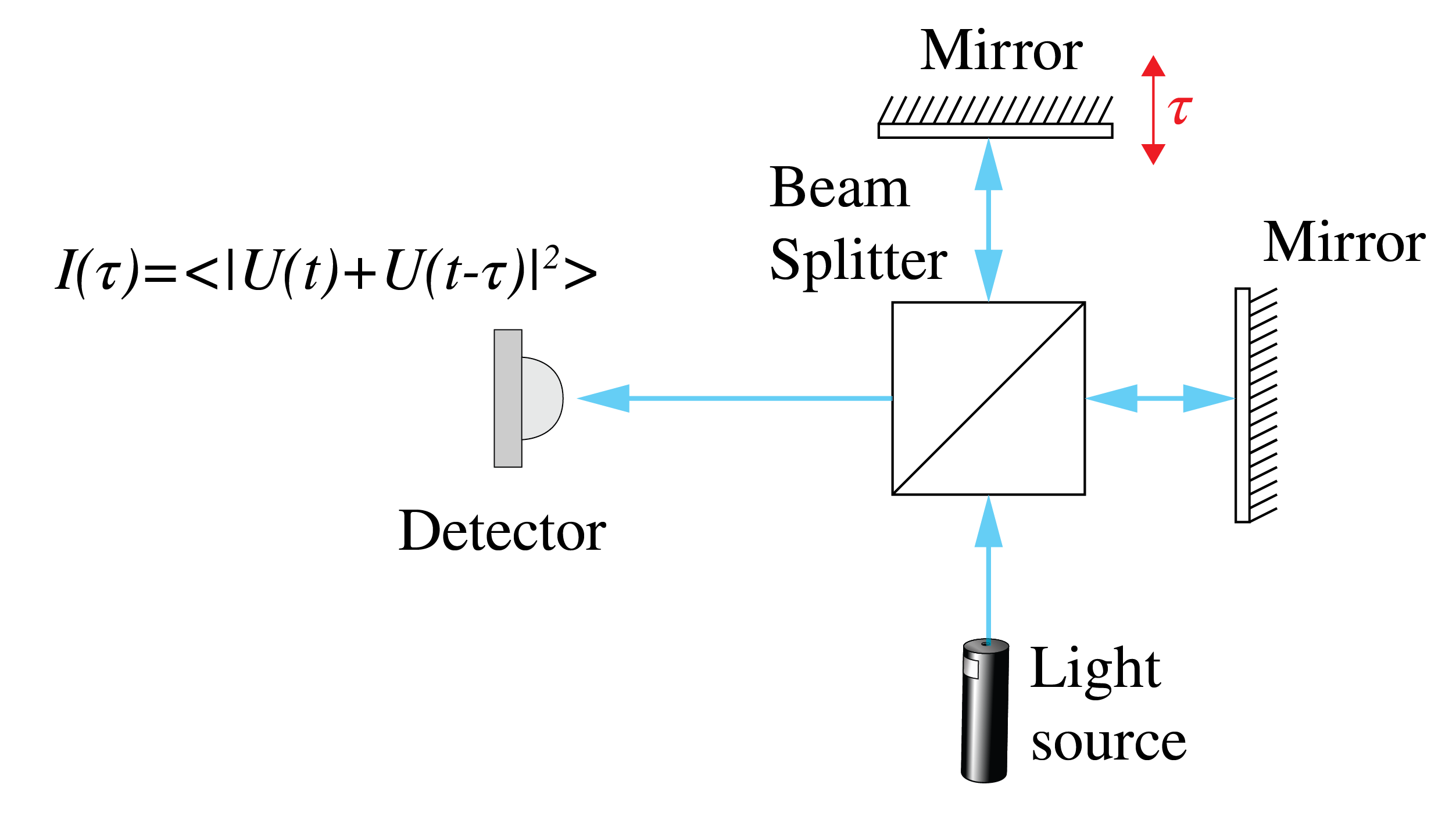
Fig. 72 A Michelson interferometer to study the temporal coherence of a field. A beam is split in two by a beam splitter, and the two beams propagate over different distances which corresponds to a time difference \(\tau\) and then interfere at the detector.

We have

(309)\[\begin{split}\begin{align*} I(\tau)&= \braket{|U(t)+U(t-\tau)|^2} &= \braket{|U(t)|^2}+\braket{|U(t-\tau)|^2}+2\text{Re} \braket{U(t)U(t-\tau)^*} \\ &= 2 \braket{|U(t)|^2} + 2\text{Re}\braket{U(t)U(t-\tau)^*}. \end{align*}\end{split}\]

The detected intensity varies with the difference in arm length.

So far we have considered a field that originates from a single atom. The total field emitted by an extended source is the sum of fields \(U_i(t)\) corresponding to all atoms \(i\). As has been explained already, the fields emitted by different atoms can not interfere. But the field emitted by an atom can interfere with the delayed field of that same atom and for every atom the interference is given by the same expression (309). The total intensity is simply that given by that of a single atom multiplied by the number of atoms. In particular, the ratio of the interference term and the other terms is the same for the entire source as for a single atom.

The self coherence function \(\Gamma(\tau)\) is defined by

\[\boxed{ \begin{align*} \Gamma(\tau)=\braket{U(t)U(t-\tau)^*} \hspace{1.5cm}\textbf{self-coherence}. \end{align*}}\]

The intensity of \(U(t)\) is

\[\begin{align*} I_0=\braket{|U(t)|^2} = \Gamma(0). \end{align*}\]

The complex degree of self-coherence is defined by:

(310)\[\boxed{\begin{align*} \gamma(\tau)=\frac{\Gamma(\tau)}{\Gamma(0)}. \hspace{1.2cm} \textbf{complex degree of self-coherence} \end{align*}}\]

Using Bessel’s inequality it can be shown that this is a complex number with modulus between \(0\) and \(1\):

(311)\[\begin{align*} 0 \leq |\gamma(\tau)| \leq 1. \end{align*}\]

The observed intensity can then be written:

(312)\[\begin{align*} I(\tau)=2 I_0 \left\{1 +\text{Re}\left[\gamma(\tau) \right]\right\}, \end{align*}\]

We consider two special cases.

1. Suppose \(U(t)\) is a monochromatic wave

\[\begin{align*} U(t)=e^{-i\omega t}. \end{align*}\]

In that case we get for the self-coherence

(313)\[\begin{align*} \begin{split} \Gamma(\tau)&=\braket{e^{-i\omega t}e^{i\omega (t-\tau)}} =e^{-i\omega \tau}, \end{split} \end{align*}\]

and

(314)\[\begin{align*} \gamma(\tau) = e^{-i\omega \tau}. \end{align*}\]

Hence the interference pattern is given by

(315)\[\begin{align*} \begin{split} I(\tau)&=2\left[1+ \cos\left( \omega\tau \right) \right]. \end{split} \end{align*}\]

So for monochromatic light we expect to detect a cosine interference pattern, which shifts as we change the arm length of the interferometer (i.e. change \(\tau\)). No matter how large the time delay \(\tau\), a clear interference pattern should be observed.

2. Next we consider what happens when the light is a superposition of two frequencies:

\[\begin{align*} U(t)=\frac{e^{-i(\mathbf{a}r{\omega}+\Delta\omega/2) t}+e^{-i(\mathbf{a}r{\omega}-\Delta\omega/2) t}}{2}, \end{align*}\]

where \(\left(2\pi/T\right) \ll \Delta \omega \ll \mathbf{a}r{\omega}\), where \(T\) is integration time of the detector. Then:

(316)\[\begin{split}\begin{align*} \Gamma(\tau)&=\frac{1}{4}\braket{\left(e^{-i(\mathbf{a}r{\omega}+\Delta\omega/2) t}+e^{-i(\mathbf{a}r{\omega}-\Delta\omega/2) t}\right)\left(e^{i(\mathbf{a}r{\omega}+\Delta\omega/2) (t-\tau)}+e^{i(\mathbf{a}r{\omega}-\Delta\omega/2) (t-\tau)}\right)} &\approx & \frac{e^{-i(\mathbf{a}r{\omega}+\Delta\omega/2) \tau}+e^{-i(\mathbf{a}r{\omega}-\Delta\omega/2) \tau}}{4} \\ &= \cos\left(\Delta\omega\,\tau/2\right)\frac{e^{-i \mathbf{a}r{\omega} \tau}}{2}, \end{align*}\end{split}\]

where in the second line the time average of terms that oscillate with time is set to zero because the averaging is done over time interval \(T\) satisfying \(T\Delta \mathbf{a}r{\omega} \gg 1\). Hence, the complex degree of self-coherence is:

(317)\[\begin{align*} \gamma(\tau)= \cos\left(\Delta\omega\,\tau/2 \right) e^{-i \mathbf{a}r{\omega} \tau} \end{align*}\]

and (312) becomes

(318)\[\begin{align*} I(\tau)= \left\{1 +\text{Re}\left[\gamma(\tau) \right]\right\}= 1 + \cos\left(\Delta\omega\,\tau/2\right) \cos(\mathbf{a}r{\omega} \tau ). \end{align*}\]

The interference term is the product of the function \(\cos(\mathbf{a}r{\omega}\tau))\), which is a rapidly oscillating function of \(\tau\), and a slowly varying envelope \(\cos \left(\Delta\omega\,\tau/2\right)\). It is interesting to note that the envelope, and hence \(\gamma(\tau)\), vanishes for some periodically spaced \(\tau\), which means that for certain \(\tau\) the degree of self-coherence vanishes and no interference fringes form ^[3].\( ^,\)^[4]. Note that when \(\Delta\omega\) is larger the intervals between the zeros of \(\gamma(\tau)\) decrease. If more frequencies are added, the envelope function is not a cosine function but on average decreases with \(\tau\). The typical value of \(\tau\) below which interferences are observed is roughly equal to half the first zero of the envelope function. This value is called the coherence time \( \Delta \tau_c\). We conclude with some further interpretations of the degree of self-coherence \(\gamma(\tau)\).

Remarks.

1. In stochastic signal analysis \(\Gamma(\tau)=\braket{U(t)U(t-\tau)^*}\) is called the autocorrelation of \(U(t)\). Informally, one can interpret the autocorrelation function as the ability to predict the field \(U\) at time \(t\) given the field at time \(t-\tau\).

2. The Wiener-Khinchin theorem says that (under the assumption of ergodicity and for stationary fields) the Fourier transform of the self coherence function is the spectral power density of \(U(t)\):

(319)\[ \hat{\Gamma}(\omega)=|\hat{U}(\omega)|^2, \]

‘Using the uncertainty principle, we can see that the larger the spread of the frequencies of \(U(t)\) (i.e. the larger the bandwidth), the more sharply peaked \(\Gamma(\tau)\) is. Thus, the light gets temporally less coherent when it consists of a broader range of frequencies. Measuring the spectral power density with a spectroscope and applying a back Fourier transform is an alternative method to obtain the complex self-coherence function.

Spatial Coherence and Young’s Experiment

Temporal coherence concerns the coherence of the field in one point. The absolute value of the degree of self coherence (310) quantifies how strong the interference is of the field in the point of interest with the field in that same point at a later time. In contrast, spatial coherence is concerned with determining how coherent the fields in two different points are. This is done by letting the fields interfere using a mask with two small holes at the positions of the points of interest and observing the fringe contrast at a distant screen (Young’s experiment).

While for temporal coherence we used a Michelson interferometer, the natural choice to characterize spatial coherence is Young’s experiment, because it allows the fields in two points \(P_1\), \(P_2\) which are separated in space to interfere with each other.

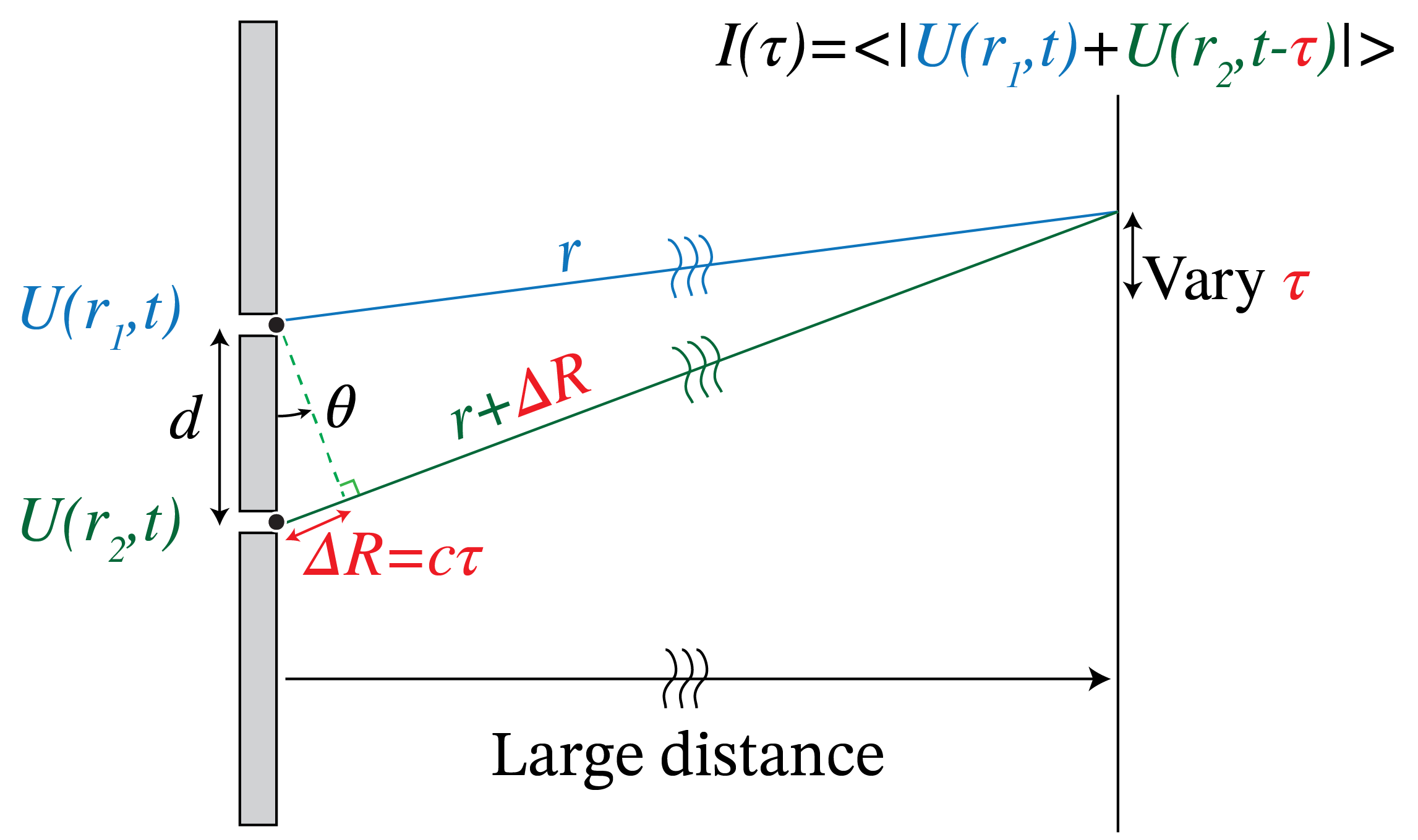
Fig. 73 Young’s experiment to evaluate the spatial coherence of two points. A mask with two holes at the two points of interest, \(\mathbf{r}_1\) and \(\mathbf{r}_2\), is used to let the fields in these points interfere with on a screen at a large distance. Because the light propagates over different distances from the two holes to the points of observation, \(U(\mathbf{r}_1,t)\) interferes with \(U(\mathbf{r}_2,t+\tau)\), where \(\tau\) is the difference in propagation time.

Let \(\mathbf{r}_1\)and \(\mathbf{r}_2\) be the position vectors of the points \(P_1\) and \(P_2\), respectively. We write the complex field in \(P_1\) as a superposition of monochromatic fields as in (304):

(320)\[\begin{align*} U(\mathbf{r}_1,t) = \int A_\omega(\mathbf{r}_1) e^{-i\omega t}\ \, \text{d} \omega. \end{align*}\]

The reason for doing this is that for a monochromatic field in the pinhole, i.e. a field with a well defined frequency, we can derive the disturbance in any point \(\mathbf{r}\) behind the mask. In fact, according to the Huygens-Fresnel Principle, a monochromatic disturbance with frequency \(\omega\) in the pinhole at \(\mathbf{r}_1\) generates a radiating spherical wave with the same frequency \(\omega\), such that in a point \(\mathbf{r}\) behind the mask the field is:

(321)\[\begin{align*} {\cal S} A_\omega(\mathbf{r}_1)\, \frac{\omega}{c} \,\frac{e^{-i \omega(t- |\mathbf{r}-\mathbf{r}_1|/c)}}{ |\mathbf{r}-\mathbf{r}_1|}, \end{align*}\]

where \({\cal S}\) is the surface area of the pinhole. We assume that the frequency band is sufficiently small such that the frequency factor that multiplies \(A_\omega\) can be replaced by the centre frequency \(\mathbf{a}r{\omega}\). Note that this should not be done in the exponent in (321) because an error in the phase can easily lead to large errors in the total field. The total field \(U_1(\mathbf{r},t)\) in \(\mathbf{r}\) due to the pinhole at \(P_1\) is obtained by integrating the monochromatic components over frequency:

(322)\[\begin{align*} U_1(\mathbf{r},t) = {\cal S} \,\frac{\mathbf{a}r{\omega}}{c} \int A_\omega(\mathbf{r}_1)\frac{e^{-i \omega( t-|\mathbf{r}-\mathbf{r}_1|/c)}}{ |\mathbf{r}-\mathbf{r}_1|} \text{d} \omega ={\cal S}\, \frac{\mathbf{a}r{\omega}}{c} \frac{U(\mathbf{r}_1, t - |\mathbf{r}-\mathbf{r}_1|/c)}{ |\mathbf{r}-\mathbf{r}_1|}. \end{align*}\]

In words:

Note

The field in \(\mathbf{r}\) at time \(t\) due to the pinhole at \(\mathbf{r}_1\) is proportional to the field at \(\mathbf{r}_1\) at the earlier time \(=|\mathbf{r}-\mathbf{r}_1|/c\) that it takes for the light to propagate form \(\mathbf{r}_1\) to \(\mathbf{r}\). The proportionality factor scales with the reciprocal distance between \(\mathbf{r}\) and \(\mathbf{r}_1\).

For the field in \(\mathbf{r}\) due to pinhole 2 we have similarly

(323)\[\begin{align*} U_2(\mathbf{r},t) = {\cal S}\, \frac{\mathbf{a}r{\omega}}{c} \frac{U(\mathbf{r}_2, t - |\mathbf{r}-\mathbf{r}_1|/c)}{ |\mathbf{r}-\mathbf{r}_2|}. \end{align*}\]

The total field in \(\mathbf{r}\) is the sum \(U_1(\mathbf{r},t)+U_2(\mathbf{r},t)\). Because of the difference in propagation distance \(\Delta R=|\mathbf{r}-\mathbf{r}_2|-|\mathbf{r}-\mathbf{r}_1|\), there is a time difference \(\tau\) between when the two fields have been emitted by the two pinholes when they arrive at a given time \(T\) IN point \(\mathbf{r}\) on the screen in Fig. 73. This time difference is given by

(324)\[\begin{align*} \tau = \frac{\Delta R}{c}. \end{align*}\]

Furthermore, the amplitudes are reduced by a factor proportional to the reciprocal distance which is different for the two fields. But if the distance of the screen to the mask is large enough, we may assumne these factors to be the same and then omit them. Using (324), the interference pattern on the screen is then, apart from a constant factor, given by

(325)\[\begin{split}\begin{align*} I(\tau)&= \braket{ \, |U_1(\mathbf{r},t) + U_2(\mathbf{r},t) |^2 \, } &= \braket{\, | U(\mathbf{r}_1, t-|\mathbf{r}-\mathbf{r}_1||/c) + U(\mathbf{r}_2, t-|\mathbf{r}-\mathbf{r}_2||/c)|^2 \, } \\ &= \braket{\, |U(\mathbf{r}_1,t)+U(\mathbf{r}_2,t- \tau)|^2\, } \\ &=\braket{\, |U(\mathbf{r}_1,t)|^2}+\braket{|U(\mathbf{r}_2,t-\tau)|^2\,}+2\text{Re}\braket{\,U(\mathbf{r}_1,t)U(\mathbf{r}_2,t-\tau)^*\, } \\ &= \braket{\, |U(\mathbf{r}_1,t)|^2\,}+\braket{\, |U(\mathbf{r}_2,t)|^2\, }+2\text{Re}\braket{\, U(\mathbf{r}_1,t)U(\mathbf{r}_2,t-\tau)^*\,}, \end{align*}\end{split}\]

where in the third and last line we used that the time average does not depend on the time it is taken because the light source is assumed to be stationary. We define the mutual coherence function by:

(326)\[\boxed{\begin{align*} \Gamma_{12}(\tau)=\braket{\,U(\mathbf{r}_1,t)U(\mathbf{r}_2,t-\tau)^*\,}, \hspace{1.5cm} \textbf{mutual coherence}. \end{align*}}\]

With the intensities

\[\begin{split}\begin{align*} \begin{split} I_1&=\braket{\, |U(\mathbf{r}_1,t)|^2\, } = \Gamma_{11}(0),\\ I_2&=\braket{\, |U(\mathbf{r}_2,t)|^2\, } = \Gamma_{22}(0). \end{split} \end{align*}\end{split}\]

the complex degree of mutual coherence is defined by

(327)\[\boxed{\begin{align*} \gamma_{12}(\tau)=\frac{\Gamma_{12}(\tau)}{\sqrt{ \Gamma_{11}(0)}\sqrt{\Gamma_{22}(0)}}, \quad \textbf{complex degree of mutual coherence}. \end{align*}}\]

It can be proved using Bessel’s inequality that

(328)\[ |\gamma_{12}(\tau)| \leq 1. \]

We can now write (325) as

\[\begin{align*} I(\tau)=I_1+I_2+2\sqrt{I_1}\sqrt{I_2}\,\text{Re} \, \gamma_{12}(\tau). \end{align*}\]

By varying the point \(\mathbf{r}\) over the screen we can vary \(\tau\) and by measuring the intensities we can determine the real part of \(\gamma_{12}(\tau)\) and hence the fringe contrast observed on the screen.

As an example, consider what happens when \(U(\mathbf{r},t)\) is a monochromatic field

\[\begin{align*} U(\mathbf{r},t)=A(\mathbf{r})e^{-i\omega t}. \end{align*}\]

In that case

\[\begin{align*} \begin{split} \Gamma_{12}(\tau)&=\braket{A(\mathbf{r}_1)A(\mathbf{r}_2)^*e^{-i\omega t}e^{i\omega (t-\tau)}} &=A(\mathbf{r}_1) A(\mathbf{r}_2)^*e^{-i\omega \tau}. \end{split} \end{align*}\]

and

(329)\[ \Gamma_{11}(0)= |A(\mathbf{r}_1)|^2, \quad \Gamma_{22}(0)=|A(\mathbf{r}_2)|^2. \]

So we get

(330)\[\begin{align*} \gamma_{12} (\tau) = \frac{\Gamma_{12}(\tau)}{|A(\mathbf{r}_1)| |A(\mathbf{r}_2)|} = e^{-i \omega \tau + i \varphi}, \end{align*}\]

where \(\varphi\) is the phase difference of \(A(\mathbf{r}_2)\) and \(A(\mathbf{r}_1)\). In this case \(\gamma_{12}\) has modulus 1, as expected for a monochromatic field. The intensity on the screen becomes

(331)\[\begin{align*} I(\tau)=|A(\mathbf{r}_1)|^2+|A(\mathbf{r}_2)|^2+2|A(\mathbf{r}_1)||A(\mathbf{r}_2)|\cos\left(\omega \tau -\varphi\right). \end{align*}\]

So indeed we see interference fringes with maximum contrast 1 and hence the fields in \(P_1\) and \(P_2\) are fully cohreent as one would expect for a monochromatic wave. If \(\varphi=0\), then interference maxima occur for

\[\begin{align*} \omega\tau=0,\pm 2\pi, \pm 4\pi, \pm 6\pi,\dots \end{align*}\]

Because \(\omega=c\frac{2\pi}{\lambda}\), and \(\Delta R=c\tau\), we find that maxima occur when

\[\begin{align*} \Delta R =0,\pm\lambda,\pm 2\lambda, \pm 3\lambda,\dots \end{align*}\]

For large distance between the screen and the mask (in the Fraunhofer limit), these path length differences correspond to directions of the maxima given by the angles \(\theta_m\) (see Fig. 73):

(332)\[\begin{align*} \theta_m = \frac{\Delta R}{d} = m \frac{\lambda}{d}, \end{align*}\]

where \(d\) is the distance between the slits and \(m\) is an integer^[5].

Remarks.

1. The mutual coherence \(\Gamma_{12}(\tau)= \braket{U(\mathbf{r}_1,t)U(\mathbf{r}_2,t-\tau)^*}\) is the cross-correlation of the two signals \(U(\mathbf{r}_1,t)\) and \(U(\mathbf{r}_2,t)\).

2. As remarked above, by moving the point of observation \(\mathbf{r}\) over the screen, one can obtain the real part of the complex degree of mutual coherence. To derive also the imaginary part, one can put a piece of glass behind one of the pinholes with thickness such that for the centre frequency \(\mathbf{a}r{\omega}\) an additional phase difference of \(\pi/2\) is obtained of the fields in \(\mathbf{r}_1\) and \(\mathbf{r}_2\). If the frequency band \(\Delta \omega\) is sufficiently narrow this phase difference applies in good approximations to all frequencies in the band.

More on Spatial Coherence

We first consider the case that the source is so small (e.g. a single emitting atom) that it can be considered to be a point source \(S\). In that case it is the fields in two points \(P_1\), \(P_2\) somewhere in space are coherent if and only if the difference in time that it takes for light to propagate from \(S\) to \(P_1\) and from \(S\) to \(P_2\) is less than the coherence time \(\Delta\tau_c\). Equivalently, for coherence the difference between the distances \(SP_1\) and \(SP_2\) must be less than the coherence length \(\Delta l_c\).

An extended classical light source consists of a large set of emitting point sources that emit by spontaneous emission. As we have explained in Coherence of Light Sources, the wave trains emitted by different atoms (point sources) in the source suffer random phase jumps due to e.g. collisions and therefore the fields emitted by different point sources in an extended classical light source can not interfere. Such a light source is called spatially incoherent. For a spatially incoherent light source, the spatial coherence in any two points \(P_1\) and \(P_2\) is determined by measuring the fringe contrast on a distance screen when a mask is used that is perpendicular to the mean direction of propagation of the light and which contains pinholes at \(P_1\) and \(P_2\). The fringe contrast and hence the mutual coherence at \(P_1\) and \(P_2\) is determined by two effects:

1. First of all it is determined by how coherent the contributions to the total field in \(P_1\) and \(P_2\) is of the individual point sources \(S\) in the extended source. This coherence is determined by the extent to which the difference between the distance of \(S\) to \(P_1\) and of \(S\) to \(P_2\) is smaller than the coherence length. If these differences in distances are for all point sources larger than the coherence length, the fringe contrast on the screen n Young’s experiment will be very low and hence the mutual coherence is very low.

2. The second effect is the size of the extended source. Even if for all point sources in the source the fields in \(P_1\) and \(P_2\) are coherent, the coherence of the total fields at \(P_1\) and \(P_2\) due to the entire source can be small. As we know, the contributions of different point sources can not interfere. Hence the intensity observed in Young’s experiment is the sum of the intensities due to the individual point sources in the extended source. The reason that the coherence of the total fields in \(P_1\) and \(P_2\) due to the entire extended source can be low even though for all point sources individually the mutual coherence in \(P_1\) and \(P_2\) is high, is that the fringe patterns due to the point sources are shifted with respect to each other which reduces the fringe contrast and hence the mutual coherence. The shift of the fringe patterns is due to the different positions in the extended source of the point sources which cause that the phase difference between the fields in \(P_1\) and \(P_2\) varies with the point sources.

We will show that when \(P_1\) and \(P_2\) have a large distance to the extended source, the two conditions mentioned above for the fields in \(P_1\) and \(P_2\) to be spatially mutually coherent are equivalently to the requirement that:

Note

The product of the angle subtended by the extended source at the midpoint of \(P_1P_2\) and the distance between \(P_1\) and \(P_2\) should be smaller than the coherence length \(\Delta l_c=c \Delta \tau_c\).

To show this we consider two mutually incoherent point sources \(S_1\) and \(S_2\) in the \(z=0\) plane. Their mutual coherence function satisfies:

(333)\[\begin{align*} \Gamma_{S_1S_2}(\tau) &= 0, \text{ for all $\tau$}, \end{align*}\]

(334)\[\begin{split}\begin{align*} \\ \Gamma_{S_1S_1}(\tau)&=\Gamma_{S_2S_2}(\tau)= \Gamma_0(\tau),\end{align*}\end{split}\]

where \(\Gamma_0\) is the self-coherence which we assume to be the same for both point sources. \(\Gamma_0(\tau)\) has width given by the coherence time \(\Delta \tau_c\) of the source and on average decreases with \(\tau\) (although not always monotonically). Eq. (333) expresses the fact that two point sources are mutually incoherent. Using that the long-time average does not depend on the origin of time which was based on the assumption that the source is stationary, we find:

(335)\[\begin{align*} \Gamma_0(-\tau)=<U(S_1,t) U(S_1,t+\tau)^*> = < U(S_1,t-\tau)U(S_1,t)^*> = \Gamma_0(\tau)^*. \end{align*}\]

Furthermore, for \(\tau=0\): \(\Gamma_0(0)=I_0\), which is the intensity of either source.

We assume for convenience that the two points \(P_1\), \(P_2\) to be at a large distance \(z\) from the two point sources and that the line \(P_1P_2\) is parallel to the extended source as shown in Fig. 74. We will compute the mutual coherence \(\Gamma_{P_1P_2}(0)\) for zero time delay \(\tau=0\) (we can also compute the mutual coherence for more general time delays \(\tau>0\), i.e. \(\Gamma_{P_1P_2}(\tau)\), but it will suffice for our purpose to take \(\tau=0\)). The fields in \(P_1\) and \(P_2\) are the sum of the fields emitted by \(S_1\) and \(S_2\). Since \(S_1\) and \(S_2\) are point sources they emit spherical waves. Therefore, similarly to (322) we find that the field in \(P_1\) is proportional to

(336)\[\begin{align*} U(P_1, t) \propto \frac{U(S_1,t-|S_1P_1|/c)}{|S_1P_1|} + \frac{U(S_2,t-|S_2P_1|/c)}{|S_2P_1|}, \end{align*}\]

and

(337)\[\begin{align*} U(P_2, t) \propto \frac{U(S_1,t-|S_1P_2|/c)}{|S_1P_2|} + \frac{U(S_2,t-|S_2P_2|/c)}{|S_2P_2|}, \end{align*}\]

where we omitted the constant factors in front of (322).

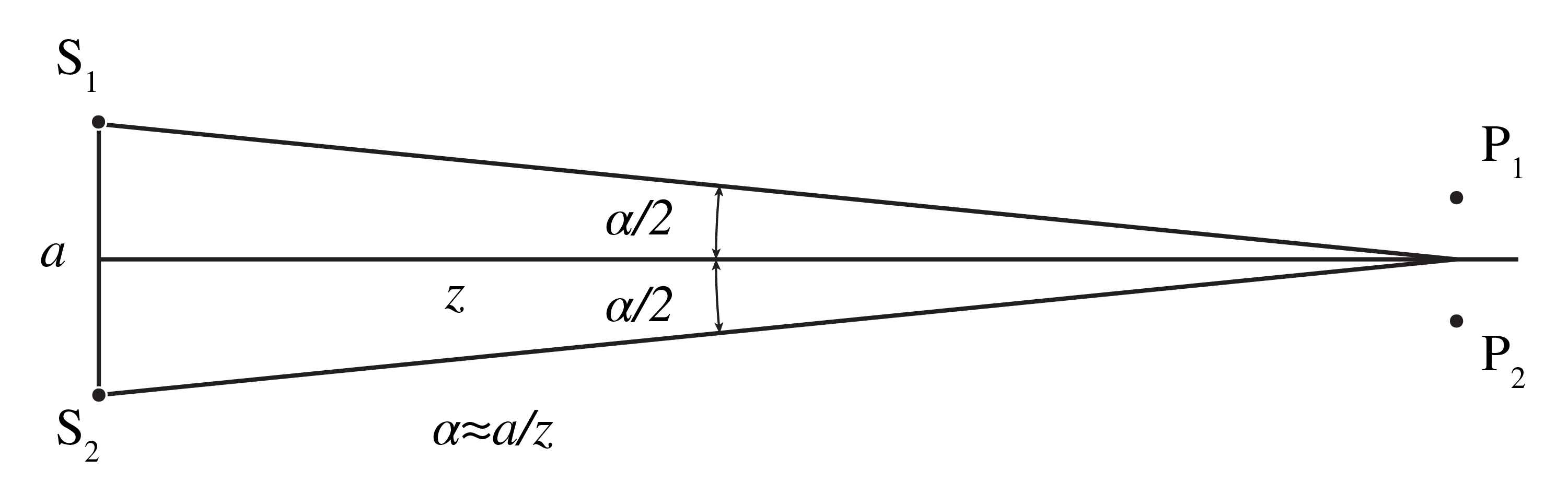
Fig. 74 Two incoherent point sources \(S_1\), \(S_2\) at a distance \(a\) from each other and two points \(P_1\), \(P_2\) in a plane at large distance \(z\) from the point sources.

For \(z\) sufficiently large all distances \(|S_iP_j|\) in the denominators may be replaced by \(z\) and then these equal distances can be omitted. By substituting (336) and (337) into (326) with \(\tau=0\), we find for the mutual coherence of \(P_1\) and \(P_2\):

(338)\[\begin{split}\begin{align*} \Gamma_{P_1P_2}(0) &= \braket{\, U(P_1,t)U(P_2,t)^*\,} \\ &= \Gamma_{S_1S_1}\left( \frac{ |S_1P_2|-|S_1P_1|}{c}\right) + \Gamma_{S_1S_2}\left( \frac{|S_2P_2|- |S_1P_1|}{c}\right) \\ & & + \Gamma_{S_2S_1}\left( \frac{|S_1P_2|-|S_2P_1|}{c}\right) + \Gamma_{S_2S_2}\left( \frac{|S_2P_2|- |S_2P_1|}{c}\right). \end{align*}\end{split}\]

Now we use (333) and (334) to get

(339)\[\begin{align*} \Gamma_{P_1P_2}(0) &= \Gamma_0\left( \frac{ |S_1P_2|-|S_1P_1|}{c}\right) + \Gamma_0\left( \frac{|S_2P_2|- |S_2P_1|}{c}\right). \end{align*}\]

Similarly,

(340)\[\begin{align*} \Gamma_{P_1P_1}(0) = \Gamma_{P_2P_2}(0)=2\Gamma_0(0)= 2I_0. \end{align*}\]

Since the width of the self coherence function \(\Gamma_0\) is the coherence time \(\Delta \tau_c\), result (339) confirms that for the fields in \(P_1\) and \(P_2\) to be coherent, the difference in distance of each of the source points to points \(P_1\) and \(P_2\) should be smaller than the coherence length \(\Delta l_c = c \Delta \tau_c \). To express the result in the angle \(\alpha\) subtended by the source at the midpoint of \(P_1P_2\) we choose coordinates such that \(P_j=(x_j,0,z)\) for \(j=1,2\). If the distance to the source is so large that \(S_1P_1\) and \(S_1P_2\) are almost parallel, we see from Fig. 75 that

(341)\[\begin{align*} |S_1P_2|-|S_1P_1|\approx |QP_2| = \frac{\alpha}{2}|x_1-x_2|. \end{align*}\]

Similarly,

(342)\[\begin{align*} |S_2P_1|-|S_2P_2|\approx \frac{\alpha}{2}|x_1-x_2|. \end{align*}\]

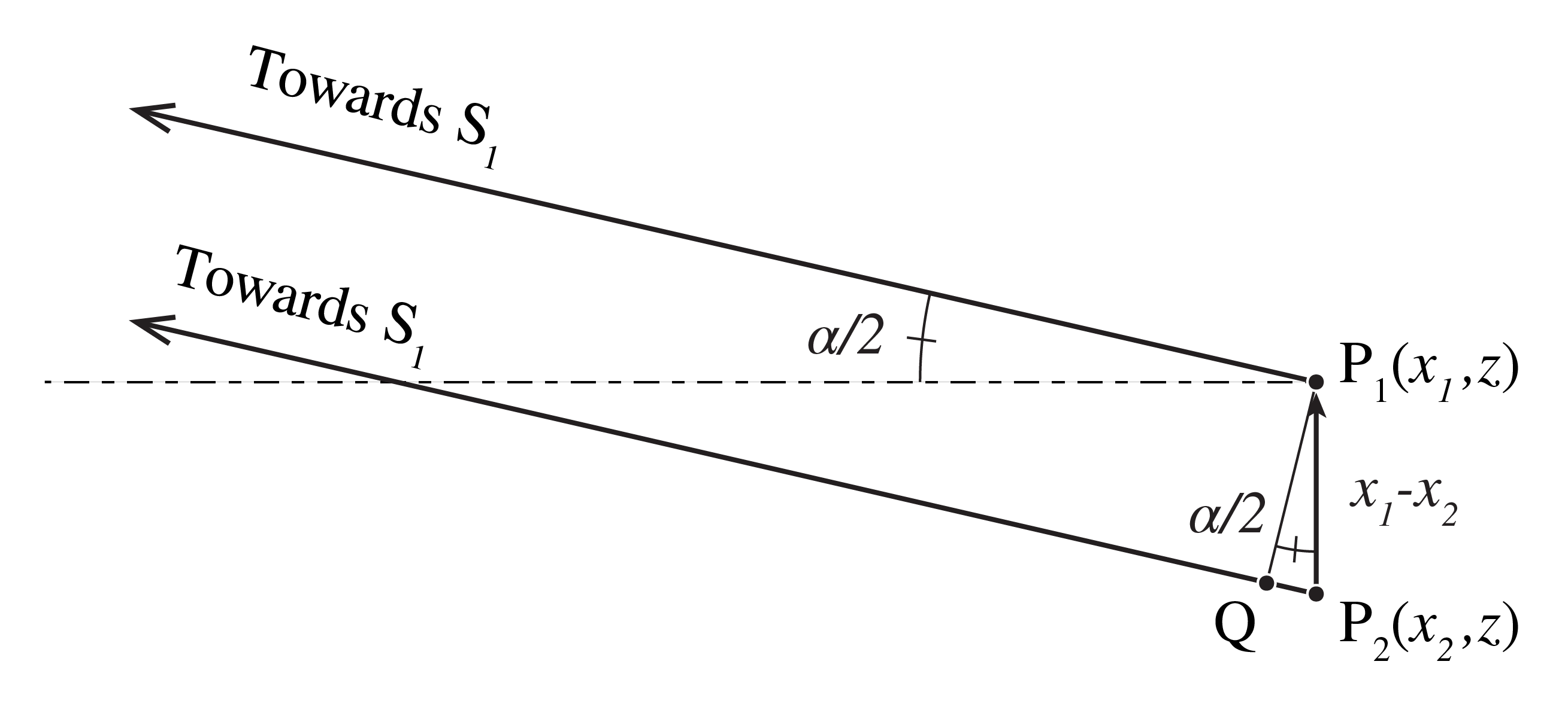
Fig. 75 For \(z\) very large, \(S_1P_1\) and \(S_1P_2\) are almost parallel and \(|S_1P_2|-|S_1P_1|\approx |QP_2|= |x_1-x_2| \alpha/2\).

Hence, with \(\Gamma_0(-\tau)=\Gamma_0(\tau)^*\), (339) becomes

(343)\[\begin{align*} \Gamma_{P_1P_2}(0) = 2\text{Re}\, \Gamma_0\left( \frac{\alpha}{2} \frac{(x_1-x_2)}{c}\right). \end{align*}\]

We conclude that for the fields in \(P_1\) and \(P_2\) to be coherent, the product of the angle \(\alpha\) which the source subtends at the midpoint of \(P_1P2\) and the distance of \(P_1P_2\) should be smaller than the coherence length \(\Delta l_c = c \Delta \tau_c\). The smaller this product is the higher the degree of spatial coherence of \(P_1\) and \(P_2\).

The angle \(\alpha\) decreases when the distance to the sources is increased and/or when the size of the source is decreased. Loosely speaking one can say that as the light propagates, it becomes more coherent. In both cases when the distance to the source increases and when the size of the source is decreased, the difference in distance of all point source to \(P_1\) and \(P_2\) decreases and will ultimately become smaller than the coherence length. Furthermore, for smaller \(\alpha\) the fringe patterns on the distant screen in Young’s experiment due to different point sources more strongly overlap which leads to a stronger overall fringe contrast.

As example consider quasi-monochromatic light for which (see (313)):

(344)\[\begin{align*} \Gamma_0(\tau) = I_0 e^{-i\mathbf{a}r{\omega}\tau}, \text{ for all $\tau$}. \end{align*}\]

where \(\mathbf{a}r{\omega}\) is the centre frequency. In this case the coherence length \(\Delta l_c\) of the source is so large that the contributions to the total field of all individual point sources are coherent. Hence the only remaining criterion for coherence of the total fields in \(P_1\) and \(P_2\) is that the fringe patterns due to the different point sources in Young’s experiment sufficiently overlap. Indeed, in this case of very long coherence time \(\Delta \tau_c\) we have

(345)\[\begin{align*} \Gamma_{P_1P_2}(0) = 2 I_0 \cos\left[\frac{\alpha}{2}\frac{\mathbf{a}r{\omega}|x_1-x_2|}{c}\right], \end{align*}\]

and hence the degree of mutual coherence is:

(346)\[\begin{split}\begin{align*} \gamma_{P_1P_2}(0) &= \frac{\Gamma_{P_1P_2}(0)}{\sqrt{\Gamma_{P_1P_1}(0)} \sqrt{\Gamma_{P_2P_2}(0)}} \\ &= \cos\left[\frac{\alpha}{2}\frac{\mathbf{a}r{\omega}|x_1-x_2|}{c}\right]. \end{align*}\end{split}\]

We see that when

(347)\[\begin{align*} |x_1-x_2| < \mathbf{a}r{\lambda}/(2 \alpha), \end{align*}\]

the fields in \(P_1\) and \(P_2\) are at least partially mutually coherent.

Example. We determine the maximum distance \(d\) between two points on earth for which sun light is coherent. The sun subtends on earth the angle:

(348)\[ \alpha = \frac{\text{AU}}{2R_\circ}\approx 0.015, \]

where \(\text{AU}\) and \(R_\circ\) are the distance of the sun to the earth and the radius of the sun. Hence, for green light \(\lambda=550 nm\) and by requiring

\[ d < \frac{\mathbf{a}r{\lambda}}{4\alpha} \nonumber \]

for appreciable mutual coherence, we find \(d_{\max}\approx 20\) micron.

Stellar Interferometry

The property that the spatial coherence of two points decreases for increasing angle which the source subtends halfway between the two points, is used in stellar interferometry. It works as follows: we want to know the size of a certain star. The size of the star, being an extended spatially incoherent source, determines the spatial coherence of the light we receive on earth. Thus, by measuring the interference of the light collected by two transversely separated telescopes, one can effectively create a double-slit experiment, with which the degree of spatial coherence of the star light on earth can be measured, and thereby the angle which the star subtends on earth. The resolution in retrieving the angle from the spatial coherence is larger when the distance between the telescopes is larger (see (346)). Then, if we know the distance of the star by independent means, e.g. from its spectral brightness, we can deduce its size from its angular size.

The method can also be used to derive the intensity distribution at the surface of the star. It can be shown that the degree of spatial coherence as function of the relative position of the telescopes is the Fourier transform of this intensity distribution. Hence, by moving the telescopes around and measuring the spatial coherence for many positions, the intensity distribution at the surface of the star can be derived from a back Fourier transform.

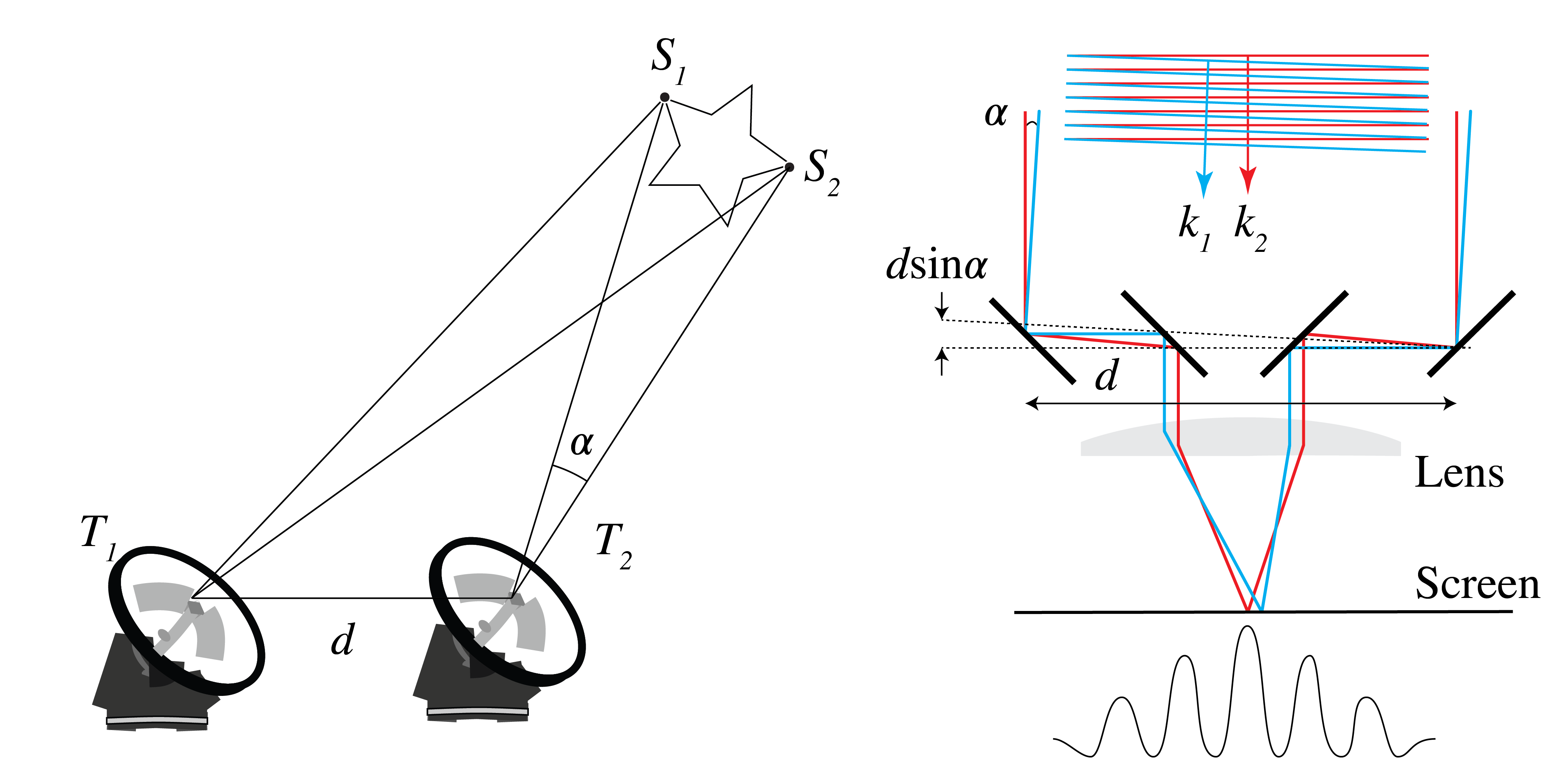
Fig. 76 Left: a stellar interferometer with two telescopes that can be moved around to measure the interference at many relative positions. Right: single telescope with two outer movable mirrors. The telescope can move around it axis. The larger the distance \(d\) the higher the resolution.

Fringe contrast

We have seen that when the interference term \(\text{Re} \braket{ U_1 U_2^* }\) vanishes, no fringes form, while when this term is nonzero, there are fringes. The fringe contrast is expressed directly in measurable intensities. Given some interference intensity pattern \(I(x)\) as in Fig. 77, the fringe contrast is defined as

\[\boxed{ \begin{align*} \mathcal{V}=\frac{I_{\text{max}}-I_{\text{min}}}{I_{\text{max}}+I_{\text{min}}}. \hspace{1.5cm} \textbf{fringe contrast}. \end{align*}}\]

For example, if we have two perfectly coherent, monochromatic point sources emitting the fields \(U_1\), \(U_2\) with intensities \(I_1=|U_1|^2\), \(I_2=|U_2|^2\), then the interference pattern is with (331):

\[\begin{align*} I(\tau)=I_1+I_2+2\sqrt{I_1 I_2}\cos(\omega \tau +\varphi). \end{align*}\]

We then get

\[\begin{align*} I_{\text{max}}=I_1+I_2+2\sqrt{I_1 I_2}, \quad I_{\text{min}}=I_1+I_2-2\sqrt{I_1 I_2}, \end{align*}\]

so

\[\begin{align*} \mathcal{V}=\frac{2\sqrt{I_1 I_2}}{I_1+I_2}. \end{align*}\]

In case \(I_1=I_2\), we find \(\mathcal{V}=1\).

In contrast, when \(U_1\) and \(U_2\) are completely incoherent, we find

\[\begin{align*} I(\tau)=I_1+I_2, \end{align*}\]

from which follows

\[\begin{align*} I_{\text{max}}=I_{\text{min}}=I_1+I_2, \end{align*}\]

which gives \(\mathcal{V}=0\).

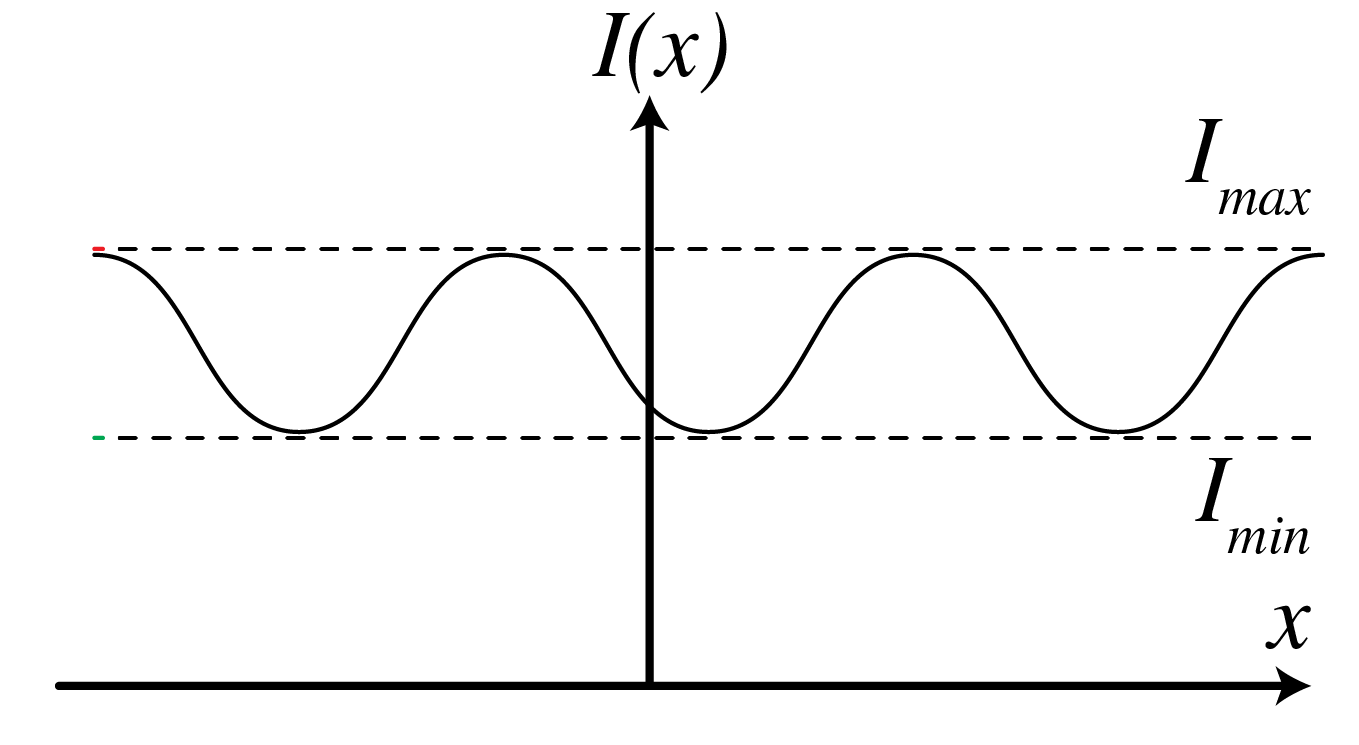
Fig. 77 Illustration of \(I_{\text{max}}\) and \(I_{\text{min}}\) of an interference pattern \(I(x)\) that determines the fringe contrast\(\mathcal{V}\).

Fabry-Perot resonator

In interferometry two mutually coherent waves are added and the intensity of the sum of the two fields is measured. This intensity contains information about the phase difference of the waves from which for example a path length difference can be deduced. One distinguishes between two types of interferometers: wavefront splitting interferometers and amplitude splitting interferometers. Examples of the first type are Young’s two slit experiment and Lloyd’s mirror (Fig. 78). Examples of amplitude splitting interferometers are the Michelson interferometer and the Fabry-Perot interferometer. The latter is not only a spectrometer of extremely high resolution but is also the resonance cavity in a laser.

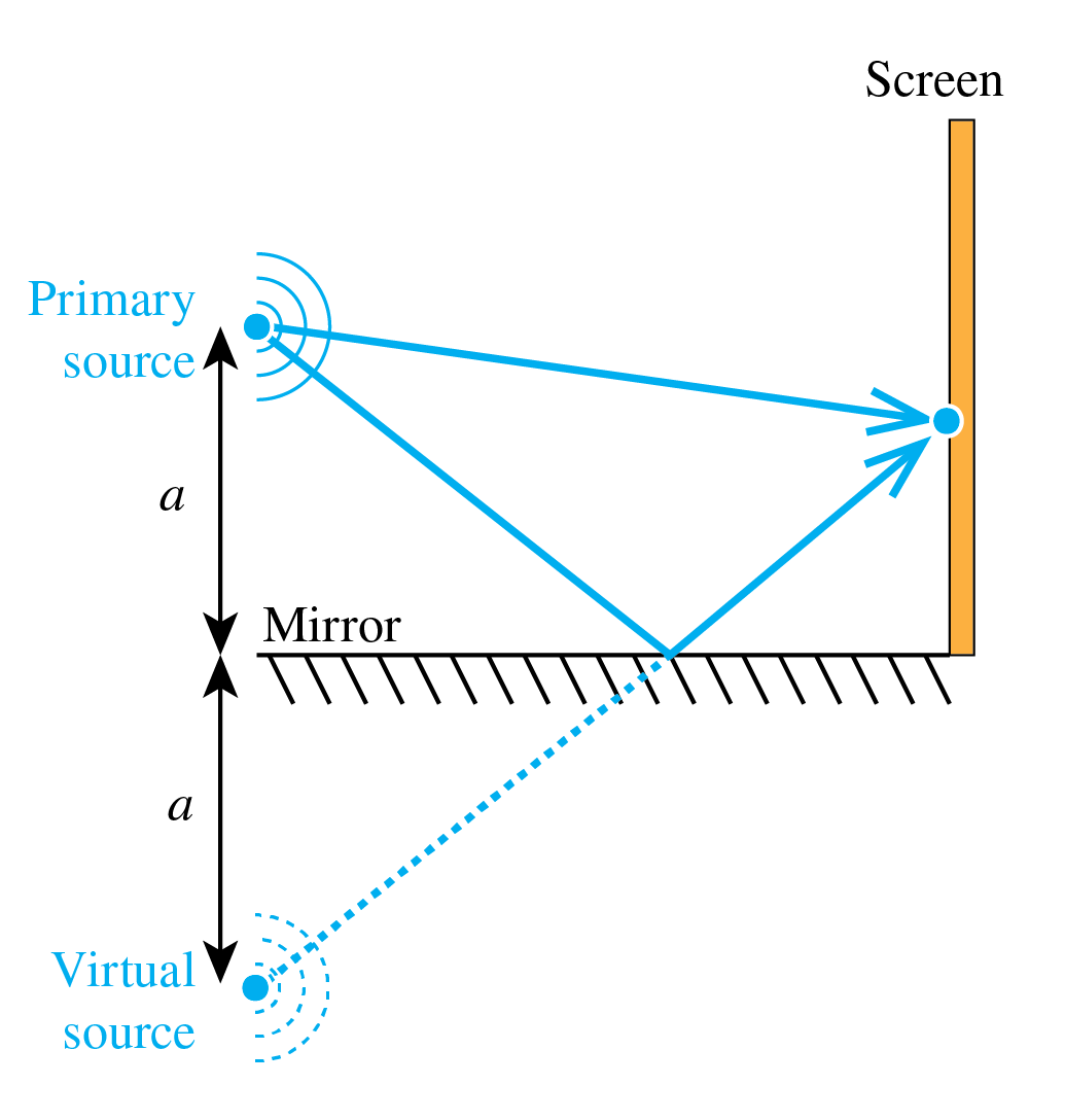
Fig. 78 Lloyd’s mirror as example of wavefront splitting interferometry.

A Fabry-Perot interferometer consists of two parallel highly reflecting surfaces with vacuum or a dielectric in between. These surfaces can be optical flats which have been coated by a metal like silver on one side. Consider a coordinate system as in Fig. 79 such that the reflecting surfaces are at \(z=0\) and \(z=d\). The refractive indices of the half spaces \(z<0\) and \(z>d\) are \(n_1\) and \(n_3\), respectively, and the refractive index of the medium between the surfaces is \(n_2\). We will first assume that all refractive indices are real.

Let there be a plane wave with unit amplitude incident from \(z<0\) under angle \(\theta_1\) with the normal as shown in Fig. 79. The incident wave is assumed to be either s- or p-polarised. There are a reflected plane wave in \(z<0\), two plane waves in medium 2 one propagating in the positive \(z\)-direction and the other in the negative \(z\)-direction and there is a transmitted plane wave in \(z>d\). It follows from the boundary conditions that the tangential component of the electric and magnetic field are continuous across the interfaces, that the tangential components of the wave vectors of all these plane waves are identical.

Let \(r_{ij}\) and \(t_{ij}\) be the reflection and transmission coefficient for a wave that is incident from medium \(i\) on the interface with medium \(j\). When the wave is s-polarised, \(r_{12}\) and \(t_{12}\) are given by Fresnel coefficients (139),(\ref{eq.ts}), whereas if the wave is p-polarised, they are given by (141), (142).

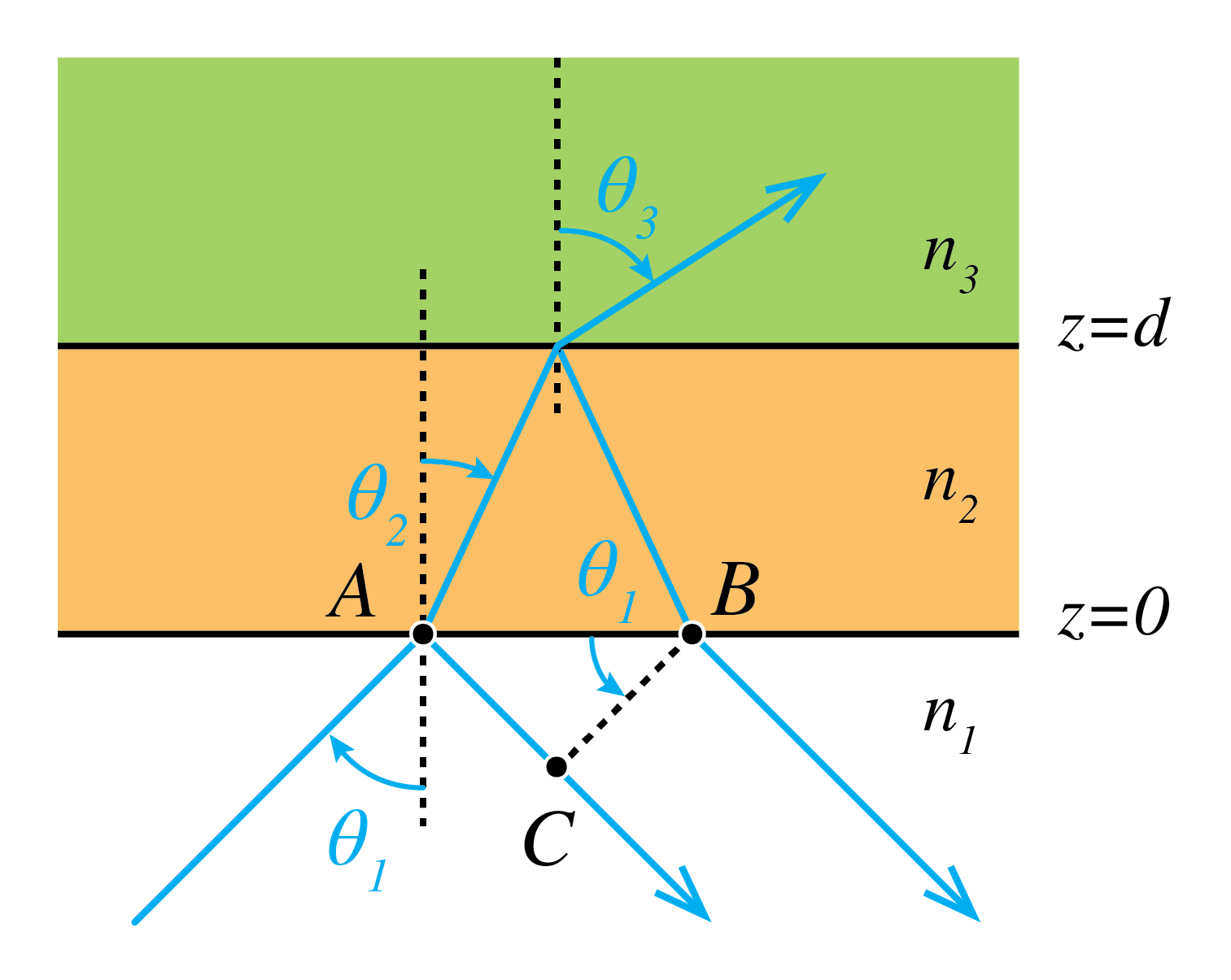
Fig. 79 Fabry-Perot with 3 layers.The light comes from the bottom and is reflected by each interface.

The incident wave, which has amplitude \(1\) in point A, is partially reflected and partially transmitted by the interface \(z=0\). The reflected wave gets amplitude \(r_{12}\). The transmitted field propagates in medium \(0<z<d\) to the interface at \(z=d\) and is then partially reflected with reflection coefficient \(r_{23}\) back to the interface \(z=0\). Because the path length inside medium 2 is \( 2d /\cos \theta_2\), the complex amplitude B of this wave in point B after transmission by the interface \(z=0\) is

(349)\[ t_{21} r_{23} t_{21} e^{ 2 i k_0 n_2 \frac{d}{\cos \theta_2}}, \]

where \(k_0\) is the wave number in vacuum. To compute the interference of the directly reflected wave and the wave that has made one round trip in medium 2, the two fields should be evaluated at the same wavefront such as wavefront CB in Fig. 79. The directly reflected field in C is obtained by propagating from B over the distance

\[\begin{split}\begin{align*} \text{AC} &= \text{AB} \sin \theta_1 \\ &= 2 d \tan\theta_2 \sin \theta_1 \\ &= 2 d \frac{n_2}{n_1 } \frac{\sin^2 \theta_2}{\cos\theta_1}. \end{align*}\end{split}\]

where Snell’s law: \(n_1 \sin\theta_1 = n_2 sin \theta_2\) has been used. Hence the total field due to the direct reflection at \(z=0\) and one round trip (349)

\[\begin{split}\begin{align*} r_{12} e^{i 2k_0 n_2 \frac{\sin^2 \theta_2}{cos \theta_2}} + t_{21} r_{23} t_{21} e^{ 2 i k_0 n_2 \frac{d}{\cos \theta_2}} \\ = e^{ i 2 k_0 n_2 d \frac{\sin^2\theta_2}{\cos\theta_2}} \left( r_{12} + t_{21}r_{23}t_{12} e^{2 i k_0 n_2d \cos \theta_2}\right). \end{align*}\end{split}\]

The common phase factor in front of the brackets may be omitted since it does not influence the reflected intensity. We then obtain

\[ r_{12} + t_{21}r_{23}t_{12} e^{2 i k^{(2)}_z d}, \]

where,

\[ k_z^{(2)}= k_0 n_2 \cos\theta_2,\]

is the \(z\)-component of the wave vector in medium 2 of the wave that propagates in the postive \(z\)-direction.

Incorporating the contributions of waves having made two or more round trips in the slab leads to the reflection coefficient of the Fabry-Perot when the field is incident from medium 1:

(350)\[\begin{split}\begin{align*} r &= r_{12} + t_{21}r_{13}t_{12} e^{2 i k^{(2)}_z d} \left[ 1 + r_{23} r_{21} e^{2 i k^{(2)}_z d} + ( r_{23} r_{21} e^{2 i k_z^{(2)} d})^2 + \ldots \right] \\ &= r_{12} + t_{21}r_{13}t_{12} e^{2 i k^{(2)}_z d}\frac{1}{ 1 - r_{23} r_{21} e^{2 i k_z^{(2)} d}} \\ &= \frac{r_{12}-r_{23} e^{2 i k^{(2)}_z d}}{1- r_{23}r_{21} e^{2 i k^{(2)}_z d}}, \end{align*}\end{split}\]

where in the last step we used

\[\begin{split}\begin{align*} t_{21}&= 1 + r_{21}, \\ t_{12}&= 1+ r_{12}, \\ r_{12}&= -r_{21} \end{align*}\end{split}\]

Similarly, the amplitude of the transmitted field in \(z=d\) gives the transmission coefficient of the Fabry-Perot when the field is incident from medium 1:

(351)\[\begin{split}\begin{align*} t &= t_{12} t_{23} e^{i k^{(2)}_z d} \left[ 1 + r_{21}r_{23} e^{2 k_z^{(2)} d} + ( r_{21}r_{23} e^{i k^{(2)}_z d})^2 + \ldots \right] \\ &= \frac{ t_{12} t_{23} e^{i k^{(2)}_z d}}{1- r_{21} r_{23} e^{ 2 i k^{(2)}_z d}}. \end{align*}\end{split}\]

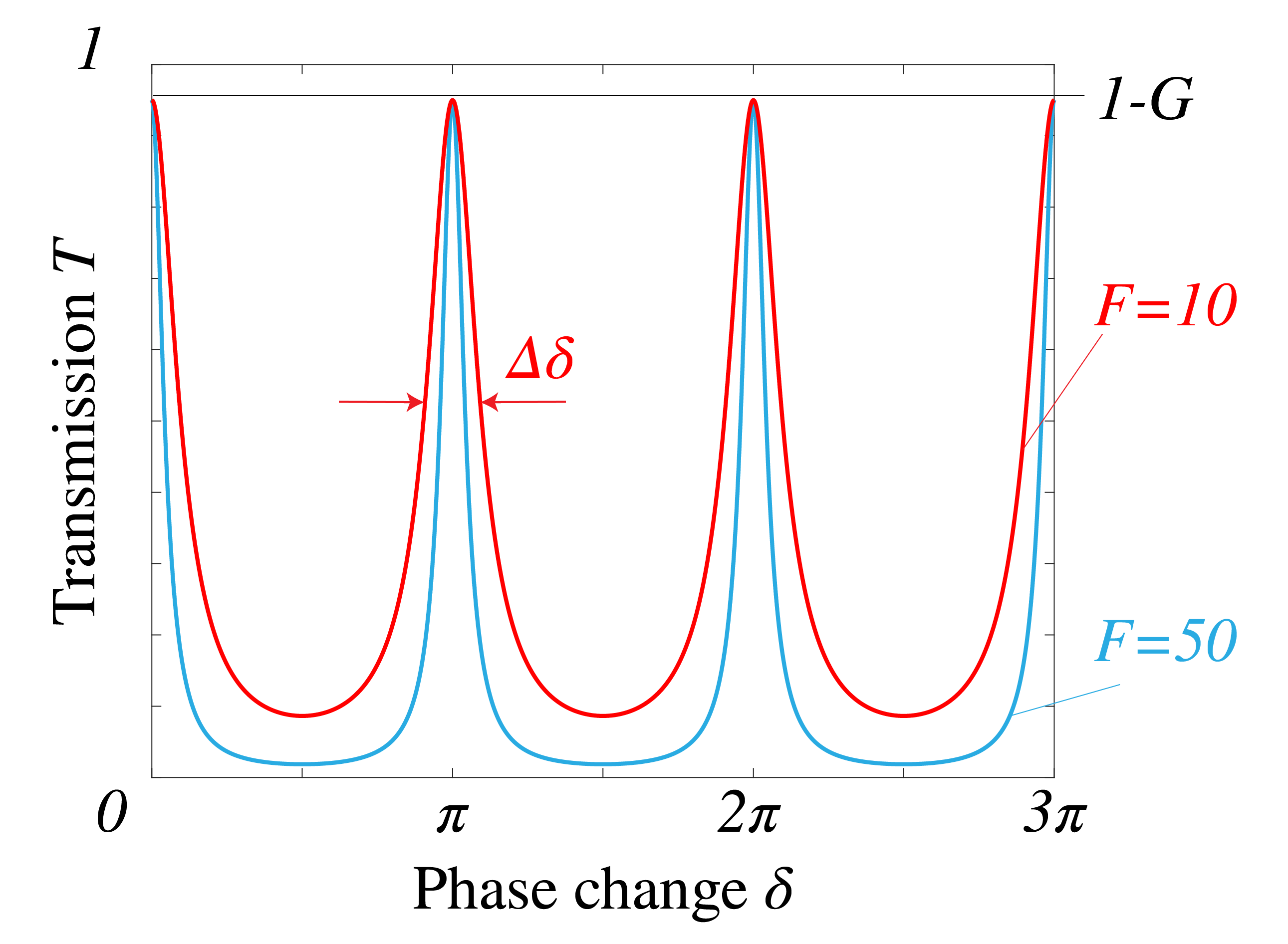
Fig. 80 Transmission coefficient versus the phase change \(\delta\) due to the Fabry-Perot. One can see the resonances occurring at every multiple of \(\pi\).

Finally, the electric field between the reflectors is given by

(352)\[\begin{split}\begin{align*} U(z) &= t_{12} e^{i k^{(2)}_z z} \left[ 1 + r_{21} r_{23} e^{2 i k^{(2)}_z d} + ( r_{21} r_{23} e^{2 i k^{(2)}_z d})^2+\ldots +\right] \\ & & + t_{12} e^{i k^{(2)}_z (d-z)}\left[ 1 + r_{21} r_{23} e^{2 i k^{(2)}_z d} + ( r_{21} r_{23} e^{2 i k^{(2)}_z d})^2+\ldots +\right] \\ &= t_{12} \frac{ e^{i k^{(2)}_z z} + r_{23} e^{i k^{(2)}_z(d-z)}} {1- r_{21} r_{23} e^{ 2 i k^{(2)}_z d}}, \end{align*}\end{split}\]

where the factor \(\exp[i(k_x x+ k_y y)]\) which gives the dependence on \((x,y)\) has been omitted.

Define

(353)\[\begin{align*} G &= \frac{(|r_{12}|-|r_{23}|)^2} {(1-|r_{23}||r_{21}|)^2}, \end{align*}\]

(354)\[\begin{split}\begin{align*} \\ F &= \frac{ 4|r_{23}||r_{21}|}{(1-|r_{23}||r_{21}|)^2}.\end{align*}\end{split}\]

\(F\) is called the coefficient of Finesse of the Fabry-Perot. It is large when the mirrors are very good reflectors. The reflected and transmitted powers, relative to the incident power are then

(355)\[ R=|r|^2 = \frac{G + F \sin^2(k^{(2)}_z d)}{1+ F \sin^2(k^{(2)}_z d)}, \]

and

(356)\[\begin{split}\begin{align*} T &= |t|^2 = 1- |R|^2 \\ &= \frac{1-G}{1+ F \sin^2(k^{(2)}_z d)}. \end{align*}\end{split}\]

We define

(357)\[ \delta = k^{(2)}_z d, \]

which is the phase change due to one pass through the middle layer of the Fabry-Perot. Then (355) and (356) become

(358)\[ R = \frac{G + F \sin^2(k^{(2)}_z d)}{1+ F \sin^2 \delta}. \]

(359)\[ T = \frac{1-G}{1+ F \sin^2 \delta}. \]

If the reflection by the mirrors is high: \(|r_{21}|\approx 1\), \(|r_{23}|\approx 1\), then \(F\) is large. This implies

(360)\[ R \approx 1, \quad T\approx 0, \]

for all \(\delta\) except when \(\sin(\delta)=0\), i.e. when

(361)\[ \delta = m\pi, \]

for some positive integer \(m\). With \(k_0=2\pi/\lambda_0\) this becomes in terms of wavelength:

(362)\[ \frac{2 d}{\lambda_0}n_2 \cos \theta_2 = m. \]

The wavelengths correspond to the maximum values of the transmission:

\[ T_{max} = 1-G. \]

and they are therefore called resonances. The width \(\Delta \delta\) at a resonance is defined as the full width at half maximum (FWHM) of the transmission, i.e.

(363)\[ \frac{1-G}{1+ \sin^2(m\pi + \Delta \delta/2)} = \frac{1}{2}(1-G), \]

which implies with \(\sin^2(m\pi + \Delta \delta/2) \approx (\Delta \delta/2)^2\):

(364)\[ \Delta \delta = \frac{2}{\sqrt{F}}. \]

Using again \(k_0=2\pi/\lambda_0\) and the fact that the width in terms of wavelength is small:

(365)\[\begin{split}\begin{align*} \frac{|\Delta \lambda_0|}{\lambda_0} &\approx & \lambda_0 \Delta\left(\frac{1}{\lambda_0}\right) \\ &= = \lambda_0 \frac{\Delta \delta}{2\pi n_2 d \cos\theta_2} \\ &= \frac{\Delta \delta}{m \pi} \\ &= \frac{2}{m \pi\sqrt{F}} \end{align*}\end{split}\]

where (362) has been used. The resolution is defined as

(366)\[ \text{Resolution} = \frac{\lambda_0}{|\Delta \lambda_0|} = \frac{m\pi \sqrt{r_{23}||r_{21}|}}{1-|r_{23}||r_{21}|}. \]

The free spectral range is the distance between adjacent resonances:

(367)\[ \Delta \delta_{free} = \pi \]

With a similar derivation as for (365)

(368)\[\begin{split}\begin{align*} \frac{|(\Delta \lambda_0)_{free}|}{\lambda_0}&\approx& -\lambda_0 \Delta\left(\frac{1}{\lambda_0}\right)_{free} \\ &= \frac{\Delta \delta_{free}}{m\pi} \\ &= \frac{1}{m}. \end{align*}\end{split}\]

A Fabry-Perot can be used as a high resolution spectrometer. Eq. (366) implies that the resolution increases for higher order \(m\). However, \(M \) can not be made arbitrary large because increasing \(m\) means according to (368) that the free spectral range decreases. The ratio

(369)\[ \frac{(\Delta \lambda_0)_{free}}{(\Delta \lambda_0) = \frac{\pi}{2} \sqrt{F}}, \]

should therefore be large.

Example. For a wavelength of \(\lambda_0=600\text{nm}\) and \(n_f d= 12 \text{mm}\) we have for normal incidence \(m=40000\). Then, if the reflection coefficients satisfy \(|r_{12}|^2=|r_{23}|^2=0.9\), we have \(F=360\) and \(G=0\). The resolution is more than one million which is better than the grating spectrometers, which will be discussed in Examples of Fresnel and Fraunhofer approximations.

Remark. Although in the derivation we have assumed that all refractive indices are real, the final formulae also apply to the case that \(n_2\) is complex. In that case \(k^{(2)}_z\) and the reflection coefficients are complex.

Interference and polarisation

In the study of interference we have so far ignored the vectorial nature of light by assuming that all the fields have the same polarisation. Suppose now that we have two real vector fields \(\mathbf{\mathcal{E}}_1\), \(\mathbf{\mathcal{E}}_2\). The (instantaneous) intensity of each field is (apart from a constant factor) given by

\[\begin{align*} \mathbf{\mathcal{E}}_1\cdot \mathbf{\mathcal{E}}_1, \quad \mathbf{\mathcal{E}}_2\cdot \mathbf{\mathcal{E}}_2. \end{align*}\]

If the two fields interfere, the instantaneous intensity is given by

(370)\[\begin{align*} (\mathbf{\mathcal{E}}_1+\mathbf{\mathcal{E}}_2)\cdot(\mathbf{\mathcal{E}}_1+\mathbf{\mathcal{E}}_2) = \mathbf{\mathcal{E}}_1\cdot \mathbf{\mathcal{E}}_1+\mathbf{\mathcal{E}}_2\cdot \mathbf{\mathcal{E}}_2+2\mathbf{\mathcal{E}}_1\cdot \mathbf{\mathcal{E}}_2, \end{align*}\]

where \(2\mathbf{\mathcal{E}}_1\cdot \mathbf{\mathcal{E}}_2\) is the interference term. Suppose the polarisation of \(\mathbf{\mathcal{E}}_1\) is orthogonal to the polarisation of \(\mathbf{\mathcal{E}}_2\), e.g.

\[\begin{split}\begin{align*} \mathbf{\mathcal{E}}_1=\begin{pmatrix}\mathcal{E}_{1x}\\ \end{pmatrix}, \quad \mathbf{\mathcal{E}}_2=\begin{pmatrix}0\\ \mathcal{E}_{2y} \\ \end{pmatrix}. \end{align*}\end{split}\]

Then \(\mathbf{\mathcal{E}}_1\cdot \mathbf{\mathcal{E}}_2=0\), which means the two fields can not interfere. This observation is the

Note

First Fresnel-Arago Law: fields with orthogonal polarisation cannot interfere.

Next we write the fields in terms of orthogonal components

\[\begin{split}\begin{align*} \mathbf{\mathcal{E}}_1=\begin{pmatrix}\mathcal{E}_{1\bot} \\ \mathcal{E}_{1\parallel}\end{pmatrix}, \quad \mathbf{\mathcal{E}}_2=\begin{pmatrix}\mathcal{E}_{2\bot} \\ \mathcal{E}_{2\parallel} \end{pmatrix}. \end{align*}\end{split}\]

This is always possible, whether the fields are polarised or randomly polarised. Then (370) becomes

\[\begin{align*} \mathbf{\mathcal{E}}_1\cdot \mathbf{\mathcal{E}}_1+\mathbf{\mathcal{E}}_2\cdot \mathbf{\mathcal{E}}_2+2\mathbf{\mathcal{E}}_1\cdot \mathbf{\mathcal{E}}_2 =\mathcal{E}_{1\bot}^2 + \mathcal{E}_{2\bot}^2 + 2\mathcal{E}_{1\bot} \mathcal{E}_{2\bot} + \mathcal{E}_{1\parallel}^2 + \mathcal{E}_{2\parallel}^2 + 2\mathcal{E}_{1\parallel} \mathcal{E}_{2\parallel}. \end{align*}\]

If the fields are randomly polarised, the time average of the \(\bot\)-part will equal the average of the \(\parallel\)-part, so the time-averaged intensity becomes

\[\begin{align*} \begin{split} I &=2\braket**calE_{1\bot**^2 + \mathcal{E}_{2\bot}^2 + 2\mathcal{E}_{1\bot} \mathcal{E}_{2\bot}} &=2\braket**calE_{1\parallel**^2 + \mathcal{E}_{2\parallel}^2 + 2\mathcal{E}_{1\parallel} \mathcal{E}_{2\parallel}}. \end{split} \end{align*}\]

This is qualitatively the same as what we would get if the fields had parallel polarisation, e.g.

\[\begin{split}\begin{align*} \mathbf{\mathcal{E}}_1=\begin{pmatrix}\mathcal{E}_{1\bot} \\ 0\end{pmatrix}, \quad \mathbf{\mathcal{E}}_2=\begin{pmatrix}\mathcal{E}_{2\bot} \\ 0\end{pmatrix}. \end{align*}\end{split}\]

This leads to the

Note

Second Fresnel-Arago Law: two fields with parallel polarisation interfere the same way as two fields that are randomly polarised.

This indicates that our initial assumption in the previous sections that all our fields have parallel polarisation is not as limiting as it may have appeared at first.

Suppose now that we have some field

\[\begin{split}\begin{align*} \mathbf{\mathcal{E}}=\begin{pmatrix}\mathcal{E}_{\bot} \\ \mathcal{E}_{\parallel}\end{pmatrix}, \end{align*}\end{split}\]

which is randomly polarised. Suppose we separate the two polarisations, and rotate one so that the two resulting fields are aligned, e.g.

\[\begin{split}\begin{align*} \mathbf{\mathcal{E}}_1=\begin{pmatrix}\mathcal{E}_{\bot} \\ 0\end{pmatrix}, \quad \mathbf{\mathcal{E}}_2=\begin{pmatrix}\mathcal{E}_{\parallel} \\ 0\end{pmatrix}. \end{align*}\end{split}\]

These fields can not interfere because \(\mathcal{E}_{\bot}\) and \(\mathcal{E}_{\parallel}\) are incoherent. This leads to the

Note

Third Fresnel-Arago Law: the two constituent orthogonal linearly polarised states of natural light cannot interfere to form a readily observable interference pattern, even if rotated into alignment.

External sources in recommended order

1. Veritasium - The original double-slit experiment, starting at 2:15 - Demonstration of an interference pattern obtained with sunlight.

2. MIT OCW - Two-beam Interference - Collimated Beams: Interference of laser light in a Michelson interferometer.

3. MIT OCW - Fringe Contrast - Path Difference: Demonstration of how fringe contrast varies with propagation distance.

4. MIT OCW - Coherence Length and Source Spectrum: Demonstration of how the coherence length depends on the spectrum of the laser light.

5. Lecture - 18 Coherence: Lecture Series on Physics - I: Oscillations and Waves by Prof. S. Bharadwaj, Department of Physics and Meteorology, IIT Kharagpur.

6. Lecture - 19 Coherence: Lecture Series on Physics - I: Oscillations and Waves by Prof. S. Bharadwaj, Department of Physics and Meteorology, IIT Kharagpur.

---

[1]

See Veritasium - The original double-slit experiment, starting at 2:15 - Demonstration of an interference pattern obtained with sunlight.

[2]

For more details see J.W. Goodman, Statistical Optics

[3]

MIT OCW - Fringe Contrast - Path Difference: Demonstration of how fringe contrast varies with propagation distance

[4]

MIT OCW - Coherence Length and Source Spectrum: Demonstration of how the coherence length depends on the spectrum of the laser light.

[5]

KhanAcademy - Young’s Double slit part 1