Basic Electromagnetic and Wave Optics

What you should know and be able to after studying this chapter

This chapter is about Maxwell’s equations and is a prerequisite for the rest of the book. It is assumed that the reader is already familiar with electromagnetism at the bachelor level. Therefore the treatments of Maxwell’s equations in matter, boundary conditions at interfaces, electromagnetic energy, the field of an electric dipole and the reflection and transmission at an interface are rather concise.

After studying this chapter you should know and be able to

• Derive the scalar wave equation for the electromagnetic field components from Maxwell’s equations.

• Work with the complex notation of time harmonic fields.

• Understand time harmonic plane waves, spherical waves and the concept of wave fronts.

• Know the main properties of the field radiated by a time-harmonic electric dipole and understand that it is the fundamental solution of Maxwell’s equations from which the radiation of any time-harmonic source can be derived.

• Qualitatively understand the far field radiation pattern of a time-harmonic electric dipole (you do not need to know the formulas).

• Derive long-time averages of products of time-harmonic functions.

• Compute the rate of energy flow using the Poynting vector and its long-time average. The derivation of the law of conservation of electromagnetic energy is not part of the exam.

• Understand the method of deriving the reflection and transmission of an incident plane wave at an interface by separating in s- and p-polarized states. The formulas for the Fresnel coefficients do not have to be known by hart.

• Understand the Brewster angle, total internal reflection and evanescent waves.

• Understand the principle of the guiding of electromagnetic waves.

Maxwell’s equations provide a very complete description of light which includes diffraction, interference and polarisation. Yet it is strictly speaking not fully accurate, because it allows monochromatic electromagnetic waves to carry any amount of energy, whereas according to quantum optics the energy is quantised. According to quantum optics, light is a flow of massless particles, the photons, which each carry an extremely small quantum of energy: \(\hbar\omega\), where \(\hbar = 6.63 \times 10^{-34}/(2\pi)\) Js and \(\omega\) is the frequency, which for visible light is of the order \(5 \times 10^{14}\) Hz. Hence for visible light \(\hbar\omega \approx 3.3\times {10^{-19}}\) J.

Quantum optics is only important in experiments involving a small number of photons, i.e. at very low light intensities and for specially prepared photons states (e.g. entangled states) for which there is no classical description. In almost all applications of optics the light sources emit so many photons that quantum effects are irrelevant see Table 1.

Table 1 The mean photon flux density for some common sources

Light Source	Number of photons/s.m\(^2\)
Laserbeam (10m W, He-Ne, focused to 20 \(\mu\)m)	\(10^{26}\)
Laserbeam (1 mW, He-Ne)	\(10^{21}\)
Bright sunlight on earth	\(10^{18}\)
Indoor light level	\(10^{16}\)
Twilight	\(10^{14}\)
Moonlight on earth	\(10^{12}\)
Starlight on earth	\(10^{10}\)

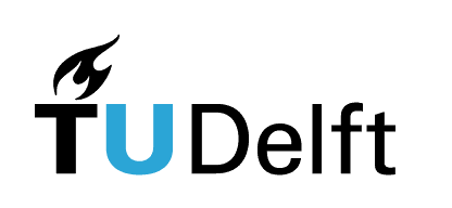
The visible part is only a small part of the overall electromagnetic spectrum (see Fig. 1). The results we will derive are however generally valid for electromagnetic waves of any frequency.

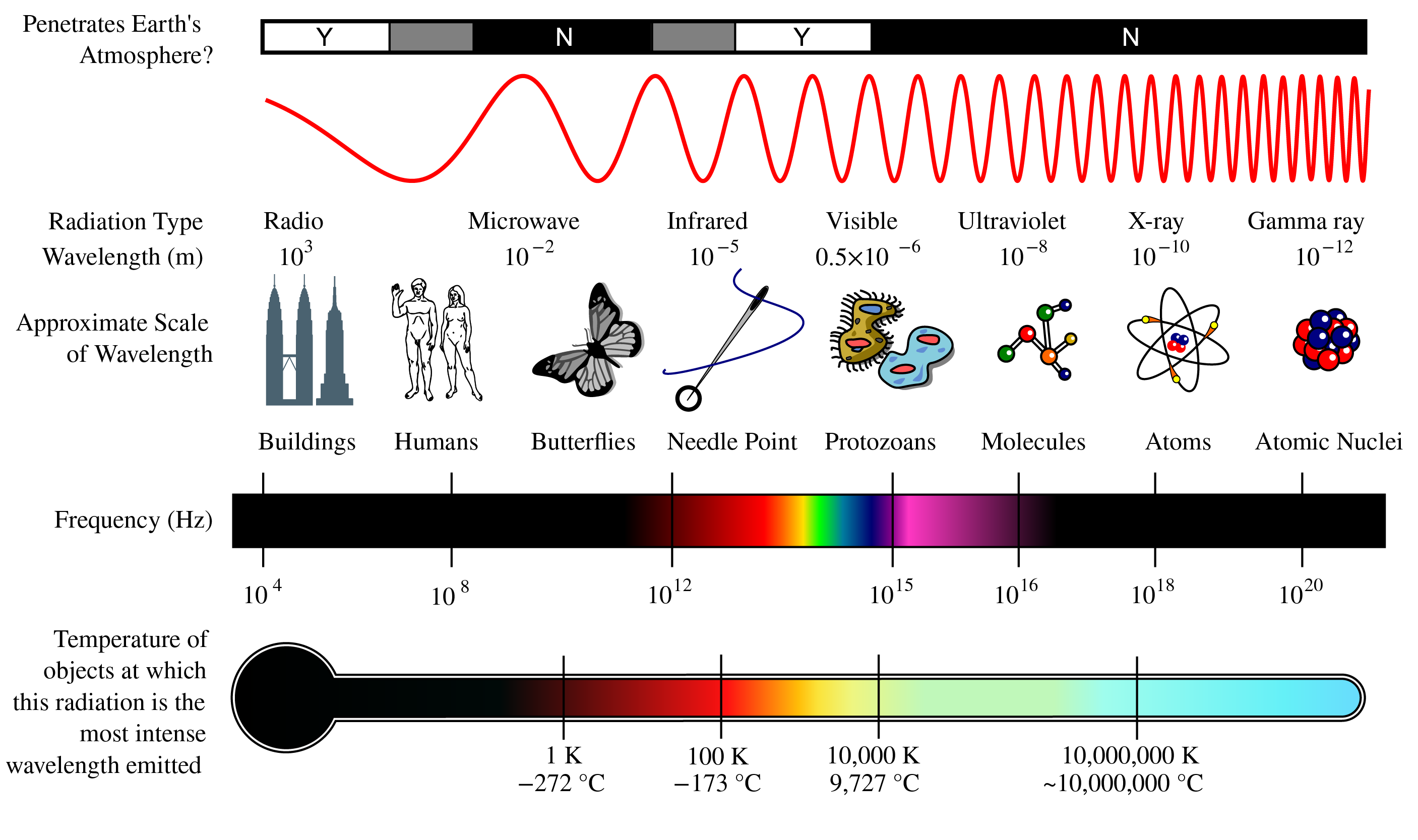
Fig. 1 The electromagnetic spectrum. (from Wikimedia Commons by NASA/ CC BY-SA ).

The Maxwell Equations in Vacuum

In a vacuum, light is described by vector fields \(\mathbf{\mathcal{E}}(\mathbf{r},t)\) [Volt/m]^[1] and \(\mathbf{\mathcal{B}}(\mathbf{r},t)\) [Tesla=Weber/\(\text{m}^2\)=g/(C.s)], which vary extremely rapidly with the position vector \(\mathbf{r}\) and time \(t\). These vector fields are traditionally called the electric field strength and the magnetic induction, respectively, and together they are referred to as “the electromagnetic field”. This terminology is explained by the fact that, because in optics these fields vary with time, the electric and magnetic fields always occur together, i.e. one does not exist without the other. Only when the fields are independent of time, there can be an electric field without a magnetic field and conversely. The first case is called electrostatics, the second magnetostatics. Time-dependent electromagnetic fields are generated by moving electric charges, the so-called sources. Let the source have charge density \(\rho(\mathbf{r},t)\) [C/\(\text{m}^3\)] and current density \(\mathbf{\mathcal{J}}(\mathbf{r},t)\) [C/(s.\(\text{m}^2\)]. Since charge can not be created nor destroyed, the rate of increase of charge inside a volume \(V\) must be equal to the flux of charges passing through its surface \(S\) from the outside to the inside of \(V\), i.e.:

(1)\[\begin{align*} \frac{d}{d t} \int_V \varrho\, \mathrm{d}V= -\int_S \mathbf{\mathcal{J}} \cdot \hat{\mathbf{n}} \, \mathrm{d}S, \end{align*}\]

where \(\hat{\mathbf{n}}\) is the outward-pointing unit normal on \(S\). Using the Gauss divergence (485), the left-hand side of (1) can be converted to a volume integral from which follows the differential form of the law of conservation of charge:

(2)\[\begin{align*} -\mathbf{\nabla} \cdot \mathbf{\mathcal{J}} = \frac{\partial \rho}{\partial t}. \end{align*}\]

At every point in space and at every time, the field vectors satisfy the Maxwell equations^[2]\(^{, }\)^[3]:

(3)\[\begin{align*} \mathbf{\nabla} \times \mathbf{\mathcal{E}} & = -\frac{\partial \mathbf{\mathcal{B}}}{\partial t}, & \text{Faraday's Law}, \end{align*}\]

(4)\[\begin{split}\begin{align*} \\ \mathbf{\nabla} \times \frac{\mathbf{\mathcal{B}}}{\mu_0} & = \epsilon_0 \frac{\partial \mathbf{\mathcal{E}}}{\partial t}+ \mathbf{\mathcal{J}}, & \text{Maxwell's Law}, \end{align*}\end{split}\]

(5)\[\begin{split}\begin{align*} \\ \mathbf{\nabla} \cdot \epsilon_0 \mathbf{\mathcal{E}} & = \varrho, & \text{Gauss's Law},\end{align*}\end{split}\]

(6)\[\begin{align*} \mathbf{\nabla} \cdot \mathbf{\mathcal{B}} & = 0, & \text{no magnetic charge}.\end{align*}\]

where \(\epsilon_0= 8.8544 \times 10^{-12}\) C \(^2\)N\(^{-1}\)m\(^{-2}\) is the dielectric permittivity and \(\mu_0 = 1.2566 \times 10^{-6} \text{m kg C}^{-2}\) is the magnetic permeability of vacuum. The quantity \(c=(1/\epsilon_0\mu_0)^{1/2}=2.997924562 \times 10^{8} \pm 1.1\) m/s is the speed of light in vacuum and \(Z=\sqrt{\mu_0/\epsilon_0}=377\Omega =377\) Vs/C is the impedance of vacuum.

Atoms are neutral and consist of a positively charged kernel surrounded by a negatively charged electron cloud. In an electric field, the centres of charge of the positive and negative charges get displaced with respect to each other. Therefore, an atom in an electric field behaves like an electric dipole. In polar molecules, the centres of charge of the positive and negative charges are permanently separated, even without an electric field. But without an electric field, they are randomly orientated and therefore have no net effect, while in the presence of an electric field they line up parallel to the field. Whatever the precise mechanism, an electric field induces a certain net dipole moment density per unit volume \(\mathbf{\mathcal{P}}(\mathbf{r})\) [C/\(\text{m}^2\)] in matter which is proportional to the local electric field \(\mathbf{\mathcal{E}}(\mathbf{r})\):

(7)\[\begin{align*} \mathbf{\mathcal{P}}(\mathbf{r},t)= \epsilon_0 \chi_e \mathbf{\mathcal{E}}(\mathbf{r},t), \end{align*}\]

where \(\chi_e\) is a dimensionless quantity, the electric susceptibility of the material. A dipole moment which varies with time radiates an electromagneticc field. It is important to realize that in (7) \(\mathbf{\mathcal{E}}\) is the total local electric field at the position of the dipole, i.e. it contains the contribution of all other dipoles, which are also excited and radiate an electromagnetic field themselves. Only in the case of diluted gasses, the influence of the other dipoles in matter can be neglected and the local electric field is simply given by the field emitted by a source external to the matter under consideration.

A dipole moment density that changes with time corresponds to a current density \(\mathbf{\mathcal{J}}_p\) [Ampere/\(\text{m}^2\)=C/(\(\text{m}^2\) s)] and a charge density \(\varrho_p\) [C/\(\text{m}^3\)] given by

(8)\[\begin{align*} \mathbf{\mathcal{J}}_p(\mathbf{r},t)&= \frac{\partial \mathbf{\mathcal{P}}(\mathbf{r},t)}{\partial t} = \epsilon_0 \chi_e \frac{\partial \mathbf{\mathcal{E}}(\mathbf{r},t)}{\partial t}, \end{align*}\]

(9)\[\begin{split}\begin{align*} \\ \varrho_p(\mathbf{r},t) &= -\mathbf{\nabla} \cdot \mathbf{\mathcal{P}}(\mathbf{r},t) =- \mathbf{\nabla} \cdot (\epsilon_0\chi_e \mathbf{\mathcal{E}}),\end{align*}\end{split}\]

All materials conduct electrons to a certain extent, although the conductivity \(\sigma\) [Ampere/(Volt m)=C/(Volt s] differs greatly between dielectrics, semi-conductors and metals (the conductivity of copper is \(10^7\) times that of a good conductor such as sea water and \(10^{19}\) times that of glass). The current density \(\mathbf{\mathcal{J}}_c\) and the charge density corresponding to the conduction electrons satisfy:

(10)\[\begin{align*} \mathbf{\mathcal{J}}_c &= \sigma \mathbf{\mathcal{E}}, \end{align*}\]

(11)\[\begin{split}\begin{align*} \\ \frac{\partial \varrho_c}{\partial t} &= -\mathbf{\nabla} \cdot \mathbf{\mathcal{J}}_c =- \mathbf{\nabla} \cdot(\sigma \mathbf{\mathcal{E}}),\end{align*}\end{split}\]

where (10) is Ohm’s Law. The total current density on the right-hand side of Maxwell’s Law (4) is the sum of \(\mathbf{\mathcal{J}}_p\), \(\mathbf{\mathcal{J}}_c\) and an external current density \(\mathbf{\mathcal{J}}_{ext}\), which we assume to be known. Similarly, the total charge density at the right of (5) is the sum of \(\varrho_p\), \(\varrho_c\) and a given external charge density \(\varrho_{ext}\). The latter is linked to the external current density by the law of conservation of charge (2). Hence, (4) and (5) become

(12)\[\begin{split}\begin{align*} \mathbf{\nabla} \times \frac{\mathbf{\mathcal{B}}}{\mu_0} &= \epsilon_0 \frac{\partial \mathbf{\mathcal{E}}}{\partial t} + \mathbf{\mathcal{J}}_p + \mathbf{\mathcal{J}}_c + \mathbf{\mathcal{J}}_{ext} \nonumber \\ &= \epsilon_0(1+\chi_e) \frac{\partial \mathbf{\mathcal{E}}}{\partial t} + \sigma \mathbf{\mathcal{E}} + \mathbf{\mathcal{J}}_{ext} \end{align*}\end{split}\]

(13)\[\begin{split}\begin{align*} \\ \mathbf{\nabla} \cdot \epsilon_0 \mathbf{\mathcal{E}} &= \varrho_p+\varrho_c + \varrho_{ext} \nonumber \\ &= - \mathbf{\nabla} \cdot (\epsilon_0 \chi_e \mathbf{\mathcal{E}}) +\varrho_c + \varrho_{ext}.\end{align*}\end{split}\]

We define the permittivity \(\epsilon\) in matter by

(14)\[\begin{align*} \epsilon= \epsilon_0(1 +\chi_e). \end{align*}\]

Then (12) and (13) can be written as

(15)\[\begin{align*} \mathbf{\nabla} \times \frac{\mathbf{\mathcal{B}}}{\mu_0} &= \epsilon \frac{\partial \mathbf{\mathcal{E}}}{\partial t} + \sigma \mathbf{\mathcal{E}} + \mathbf{\mathcal{J}}_{ext} \end{align*}\]

(16)\[\begin{split}\begin{align*} \\ \mathbf{\nabla}\cdot (\epsilon \mathbf{\mathcal{E}}) &= \varrho_c + \varrho_{ext}.\end{align*}\end{split}\]

It is verified in Problem 1 that in a conductor any accumulation of charge is extremely quickly reduced to zero. Therefore we may assume that

(17)\[\begin{align*} \varrho_c=0. \end{align*}\]

If the material is magnetic, the magnetic permeability is different from vacuum and is written as \(\mu=\mu_0(1+\chi_m)\), where \(\chi_m\) is the magnetic susceptibility. In the Maxwell equations, one should then replace \(\mu_0\) by \(\mu\). However, at optical frequencies magnetic effects are negligible (except in ferromagnetic materials, which are rare). We will therefore always assume that the magnetic permeability is that of vacuum: \(\mu=\mu_0\).

It is customary to define the magnetic field by \(\mathbf{\mathcal{H}}=\mathbf{\mathcal{B}}/\mu_0\) [Ampere/m=C/(ms)]. By using the magnetic field \(\mathbf{\mathcal{H}}\) instead of the magnetic induction \(\mathbf{\mathcal{B}}\), Maxwell’s equations become more symmetric:

(18)\[\begin{align*} \mathbf{\nabla} \times \mathbf{\mathcal{E}} & = -\mu_0 \frac{\partial \mathbf{\mathcal{H}}}{\partial t }, & \text{Faraday's Law} \end{align*}\]

(19)\[\begin{split}\begin{align*} , \\ \mathbf{\nabla} \times \mathbf{\mathcal{H}} & = \epsilon \frac{\partial \mathbf{\mathcal{E}}}{\partial t} + \sigma \mathbf{\mathcal{E}}+ \mathbf{\mathcal{J}}_{ext}, & \text{Maxwell's Law}, \end{align*}\end{split}\]

(20)\[\begin{split}\begin{align*} \\ \mathbf{\nabla} \cdot \epsilon \mathbf{\mathcal{E}} & = \varrho_{ext}, & \text{Gauss's Law}, \end{align*}\end{split}\]

(21)\[\begin{split}\begin{align*} \\ \mathbf{\nabla} \cdot \mathbf{\mathcal{H}} & = 0. & \text{no magnetic charge}.\end{align*}\end{split}\]

This is the form in which we will be using the Maxwell equations in matter in this book. It is seen that the Maxwell equations in matter are identical to those in vacuum, with \(\epsilon\) substituted for \(\epsilon_0\).

We end this section with remarking that our derivations are valid for non-magnetic materials which are electrically isotropic. This means that the magnetic permeability is that of vacuum and that the permittivity \(\epsilon\) is a scalar. In an anisotropic dielectric the induced dipole vectors are in general not parallel to the local electric field. Then \(\chi_e\) and therefore also \(\epsilon\) become matrices. Throughout this book all matter is assumed to be non-magnetic and electrically isotropic.

We consider a homogeneous insulator (i.e. \(\epsilon\) is independent of position and \(\sigma\)=0) in which there are no external sources:

(22)\[\begin{align*} \mathbf{\mathcal{J}}_{ext}=0, \;\; \varrho_{ext}=0. \end{align*}\]

In optics the external source, e.g. a laser, is normally spatially separated from the objects of interest with which the light interacts. Therefore the assumption that the external source vanishes in the region of interest is often justified. Take the curl of (18) and the time derivative of (19) and add the equations obtained. This gives

(23)\[\begin{align*} \mathbf{\nabla} \times \mathbf{\nabla} \times \mathbf{\mathcal{E}} + \epsilon \mu_0 \frac{\partial^2 \mathbf{\mathcal{E}}}{\partial t^2}=\mathbf{0}. \end{align*}\]

Now for any vector field \(\mathbf{\mathcal{A}}\) there holds:

(24)\[\begin{align*} \mathbf{\nabla} \times \mathbf{\nabla} \times \mathbf{\mathcal{A}} = - \mathbf{\nabla}^2 \mathbf{\mathcal{A}} + \mathbf{\nabla} \mathbf{\nabla} \cdot \mathbf{\mathcal{A}}. \end{align*}\]

where \(\mathbf{\nabla}^2 \mathbf{\mathcal{A}}\) is the vector:

(25)\[\begin{align*} \mathbf{\nabla}^2 \mathbf{\mathcal{A}} = \mathbf{\nabla}^2 {\cal A}_x \, \hat{\mathbf{x}} + \mathbf{\nabla}^2 {\cal A}_y \, \hat{\mathbf{y}} + \mathbf{\nabla}^2 {\cal A}_z \, \hat{\mathbf{z}}, \end{align*}\]

with

(26)\[\begin{align*} \mathbf{\nabla}^2 = \frac{\partial^2}{\partial x^2} + \frac{\partial^2}{\partial y^2} + \frac{\partial^2}{\partial z^2}. \end{align*}\]

Because Gauss’s law (20) with \(\varrho_{ext}=0\) and \(\epsilon\) constant implies that \(\mathbf{\nabla}\cdot \mathbf{\mathcal{E}}=0\), (24) applied to \(\mathbf{\mathcal{E}}\) yields

(27)\[\begin{align*} \mathbf{\nabla} \times \mathbf{\nabla} \times \mathbf{\mathcal{E}} = - \mathbf{\nabla}^2 \mathbf{\mathcal{E}}. \end{align*}\]

Hence, (23) becomes

(28)\[\begin{align*} \mathbf{\nabla}^2 \mathbf{\mathcal{E}} - \epsilon \mu_0 \frac{\partial^2 \mathbf{\mathcal{E}}}{\partial t^2}=\mathbf{0}. \end{align*}\]

By a similar derivation it is found that also \(\mathbf{\mathcal{H}}\) satisfies (28). Hence in a homogeneous dielectric without external sources, every component of the electromagnetic field satisfies the scalar wave equation:

(29)\[\begin{align*} \mathbf{\nabla}^2 {\cal U} - \epsilon \mu_0 \frac{\partial^2 {\cal U}}{\partial t^2}=0. \end{align*}\]

The refractive index is the dimensionless quantity defined by

(30)\[\begin{align*} n = \sqrt{\frac{\epsilon}{\epsilon_0}}. \end{align*}\]

The scalar wave equation can then be written as

(31)\[\begin{align*} \mathbf{\nabla}^2 {\cal U} - n^2 \epsilon_0 \mu_0 \frac{\partial^2 {\cal U}}{\partial t^2}=0. \end{align*}\]

The speed of light in matter is

(32)\[\begin{align*} \frac{c}{n}=\frac{1}{\sqrt{\epsilon \mu_0}}. \end{align*}\]

Time-Harmonic Solutions of the Wave Equation

The fact that, in the frequently occurring circumstance in which light interacts with a homogeneous dielectric, all components of the electromagnetic field satisfy the scalar wave equation, justifies the study of solutions of this equation. Since in most cases in optics monochromatic fields are considered, we will focus our attention on time-harmonic solutions of the wave equation.

Time-Harmonic Plane Waves

Time-harmonic solutions depend on time by a cosine or a sine function. One can easily verify by substitution that

(33)\[\begin{align*} {\cal U}(\mathbf{r},t) ={\cal A} \cos(kx - \omega t + \varphi), \end{align*}\]

where \({\cal A}>0\) and \(\varphi\) are constants, is a solution of (31), provided that

(34)\[\begin{align*} k = \omega (\epsilon \mu_0)^{1/2} = \omega n \sqrt{\epsilon_0 \mu_0}= n k_0, \end{align*}\]

where \(k_0=\omega \sqrt{\epsilon_0 \mu_0}\) is the wave number in vacuum. The frequency \(\omega>0\) can be chosen arbitrarily. The wave number \(k\) in the material is then determined by (34). We define \(T=2\pi/\omega\) and \(\lambda=2\pi/k\) as the period and the wavelength in the material, respectively. Furthermore, \(\lambda_0=2\pi/k_0\) is the wavelength in vacuum.

Remark. With “the wavelength”, we always mean the wavelength in vacuum.

We can write (33) in the form

(35)\[\begin{align*} {\cal U}(x,t)={\cal A}\cos\left[k\left(x-\frac{c}{n} t\right)+\varphi\right], \end{align*}\]

where \(c/n=1/\sqrt{\epsilon\mu_0}\) is the speed of light in the material. \({\cal A}\) is the amplitude and the argument under the cosine: \(k\left(x-\frac{c}{n} t\right)+\varphi\) is called the phase at position \(x\) and at time \(t\). A wave front is a set of space-time points where the phase is constant:

\[\begin{align*} x - \frac{c}{n} t =\text{constant}. \end{align*}\]

At any fixed time \(t\) the wave fronts are planes (in this case perpendicular to the \(x\)-axis), and therefore the wave is called a plane wave. As time proceeds, the wave fronts move with velocity \(c/n\) in the positive \(x\)-direction.

A time-harmonic plane wave propagating in an arbitrary direction is given by

(36)\[\begin{align*} {\cal U}(\mathbf{r},t) ={\cal A} \cos( \mathbf{k}\cdot \mathbf{r} -\omega t + \varphi), \end{align*}\]

where \({\cal A}\) and \(\varphi\) are again constants and \(\mathbf{k}=k_x\hat{\mathbf{x}}+k_y \hat{\mathbf{y}}+k_z \hat{\mathbf{z}}\) is the wave vector. The wave fronts are given by the set of all space-time points \((\mathbf{r}, t)\) for which the phase \(\mathbf{k}\cdot \mathbf{r} -\omega t + \varphi\) is constant, i.e. for which

(37)\[\begin{align*} \mathbf{k}\cdot \mathbf{r} -\omega t =\text{constant}. \end{align*}\]

At fixed times the wave fronts are planes perpendicular to the direction of \(\mathbf{k}\) as shown in Fig. 2. Eq. (36) is a solution of (31) provided that

(38)\[\begin{align*} k_x^2 + k_y^2 + k_z^2 = \omega^2 \epsilon \mu_0 = \omega^2 n^2 \epsilon_0 \mu_0=k_0^2n^2. \end{align*}\]

The direction of the wave vector can be chosen arbitrarily, but its length is determined by the frequency \(\omega\).

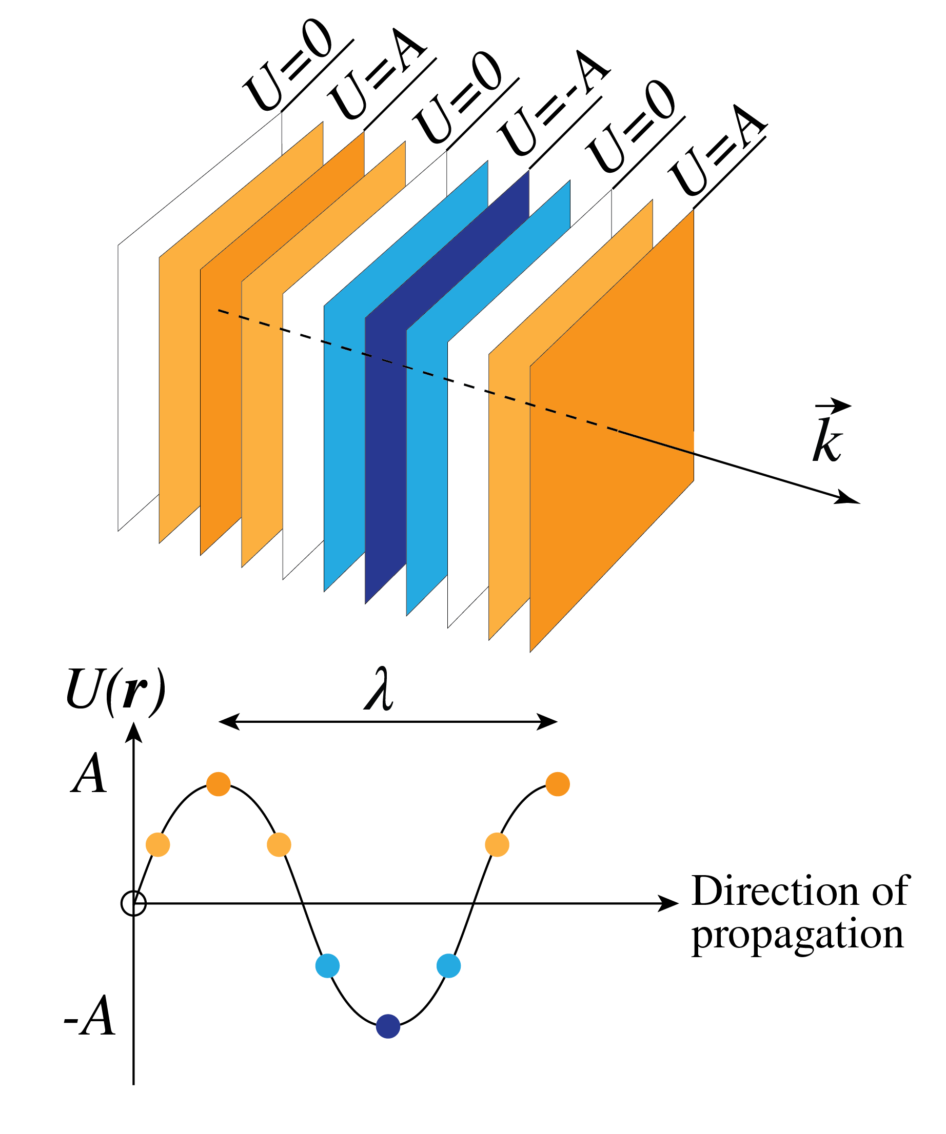
Fig. 2 Planes of constant phase.

We consider a general time-harmonic solution of the wave equation (29):

(39)\[\begin{align*} {\cal U}(\mathbf{r},t) = {\cal A}(\mathbf{r}) \cos(\varphi(\mathbf{r})- \omega t), \end{align*}\]

where the amplitude \({\cal A}(\mathbf{r})>0\) and the phase \(\varphi(\mathbf{r})\) are functions of position \(\mathbf{r}\). The wave fronts consist of sets of space-time points \((\mathbf{r},t)\) where the phase is equal to some constant:

(40)\[\begin{align*} \varphi(\mathbf{r})- \omega t=\text{constant}. \end{align*}\]

At fixed time \(t\), the sets of constant phase: \(\varphi(\mathbf{r})=\omega t + \text{constant}\) are surfaces which in general are not planes, hence the solution in general is not a plane wave. Eq. (39) could for example be a wave with spherical wave fronts, as discussed below.

Remark. A plane wave is infinitely extended and transports an infinite amount of electromagnetic energy. A plane plane can therefore not exist in reality, but it is nevertheless a usual idealisation. As will be demonstrated in Section 7.1, every time-harmonic solution of the wave equation can always be expanded in terms of plane waves of the form (36).

For time-harmonic solutions it is often convenient to use complex notation. Define the complex amplitude by:

(41)\[\begin{align*} U(\mathbf{r}) = {\cal A}(\mathbf{r}) e^{i\varphi(\mathbf{r})}, \end{align*}\]

i.e. the modulus of the complex number \(U(\mathbf{r})\) is the amplitude \({\cal A}(\mathbf{r})\) and the argument of \(U(\mathbf{r})\) is the phase \(\varphi(\mathbf{r})\) at \(t=0\). The time-dependent part of the phase: \(-\omega t\) is thus separated from the space-dependent part of the phase. Then (39) can be written as

(42)\[\begin{align*} {\cal U}(\mathbf{r},t) = \text{Re}\left[ U(\mathbf{r}) e^{-i\omega t} \right]. \end{align*}\]

Hence \({\cal U}(\mathbf{r},t)\) is the real part of the complex time-harmonic function

(43)\[\begin{align*} U(\mathbf{r}) e^{-i\omega t}. \end{align*}\]

Remark. The complex amplitude \(U(\mathbf{r})\) is also called the complex field. In the case of vector fields such as \(\mathbf{E}\) and \(\mathbf{H}\) we speak of complex vector fields, or simply complex fields. Complex amplitudes and complex (vector) fields are only functions of position \(\mathbf{r}\); the time dependent factor \(\exp(-i\omega t)\) is omitted. To get the physical meaningful real quantity, the complex amplitude or complex field first has to be multiplied by \(\exp(-i\omega t)\) and then the real part must be taken.

The following convention is used throughout this book:

Real-valued physical quantities (whether they are time-harmonic or have more general time dependence) are denoted by a calligraphic letter, e.g. \(\mathcal{U}\), \(\mathcal{E}_x\), or \(\mathcal{H}_x\). The symbols are bold when we are dealing with a vector, e.g. \(\mathbf{\mathcal{E}}\) or \(\mathbf{\mathcal{H}}\). The complex amplitude of a time-harmonic function is linked to the real physical quantity by (42) and is written as an ordinary letter such as \(U\) and \(\mathbf{E}\).

It is easier to calculate with complex amplitudes (complex fields) than with trigonometric functions (cosine and sine). As long as all the operations carried out on the functions are linear, the operations can be carried out on the complex quantities. To get the real-valued physical quantity of the result (i.e. the physical meaningful result), multiply the finally obtained complex amplitude by \(\exp(-i\omega t)\) and take the real part. The reason that this works is that taking the real part commutes with all linear operations, i.e. taking first the real part to get the real-valued physical quantity and then operating on this real physical quantity gives the same result as operating on the complex scalar and taking the real part at the end.

By substituting (42) into the wave equation (31) we get

(44)\[\begin{split}\begin{align*} \nabla^2 {\cal U}(\mathbf{r},t) - n^2 \epsilon_0\mu_0 \frac{\partial^2{\cal U}(\mathbf{r},t)}{\partial t^2} &= \text{Re}\left[ \nabla^2 U(\mathbf{r})e^{-i\omega t}\right] - n^2 \epsilon_0\mu_0 \text{Re}\left[ U(\mathbf{r})\frac{\partial^2 e^{-i\omega t}}{\partial ^2}\right] \\ &= \text{Re}\left\{ \left[\nabla^2 U(\mathbf{r}) + \omega^2 n^2 \epsilon_0\mu_0 U(\mathbf{r}) \right] e^{-i\omega t}\right\}. \end{align*}\end{split}\]

Since this must vanish for all times \(t\), it follows that the complex expression between the brackets \(\{.\}\) must vanish. To see this, consider for example the two instances \(t=0\) and \(t=\pi/(2\omega\). We conclude that the complex amplitude satisfies

(45)\[\boxed{\begin{align*} \nabla^2 U(\mathbf{r}) + k_0^2 n^2 U(\mathbf{r})=0,\quad \text{Helmholtz Equation}, \end{align*}}\]

where \(k_0=\omega \sqrt{\epsilon_0 \mu_0}\) is the wave number in vacuum.

Remark. The complex quantity of which the real part has to be taken is: \(U\exp(-i\omega t)\). As explained above, it is not necessary to drag the time-dependent factor \(\exp(-i \omega t )\) along in the computations: it suffices to calculate only with the complex amplitude \(U\), then multiply by \(\exp(-i\omega t)\) and then take the real part. However, when a derivative with respect to time has to be taken: \(\partial /\partial t\), the complex field much be multiplied by \(-i\omega\). This is also done in the time-harmonic Maxwell’s equations in Time-Harmonic Maxwell Equations in Matter below.

Time-Harmonic Spherical Waves

A spherical wave depends on position only by the distance to a fixed point. For simplicity we choose the origin of our coordinate system at this point. We thus seek a solution of the form \({\cal U}(r,t)\) with \(r=\sqrt{x^2+y^2+z^2}\). For spherical symmetric functions we have

(46)\[\begin{align*} \mathbf{\nabla}^2 {\cal U}(r,t) = \frac{1}{r} \frac{\partial^2}{\partial r^2}[ r {\cal U}(r,t)]. \end{align*}\]

It is easy to see that outside of the origin

(47)\[\begin{align*} {\cal U}(r,t) = \frac{f( \pm r - ct/n )}{r}, \end{align*}\]

satisfies (46) for any choice for the function \(f\), where as before \(c=1/\sqrt{\epsilon_0\mu_0}\) is the speed of light and \(n=\sqrt{\epsilon/\epsilon_0}\). Of particular interest are time-harmonic spherical waves:

(48)\[\begin{align*} {\cal U}(r, t) = \frac{{\cal A}}{r} \cos\left[ k\left( \pm r - \frac{c}{n} t\right) + \varphi \right] = \frac{{\cal A}}{r} \cos[ \pm k r- \omega t + \varphi ) \end{align*}\]

where \({\cal A}\) is a constant

(49)\[\begin{align*} k= n \omega/c. \end{align*}\]

and \(\pm kr - \omega t +\varphi\) is the phase at \(\mathbf{r}\) and at time \(t\). A wave front is a set of space-time points \((\mathbf{r},t)\) where the phase is equal to a constant:

(50)\[\begin{align*} \pm k r - \omega t = \text{constant}. \end{align*}\]

Wave fronts are thus spheres which move with the speed of light in the radial direction. When the \(+\) sign is chosen, the wave propagates outwards, i.e. away from the origin. The wave is then radiated by a source at the origin. Indeed, if the \(+\) sign holds in (48), then if time \(t\) increases, (50) implies that a surface of constant phase moves outwards. Similarly, if the \(-\) sign holds, the wave propagates towards the origin which then acts as a sink.

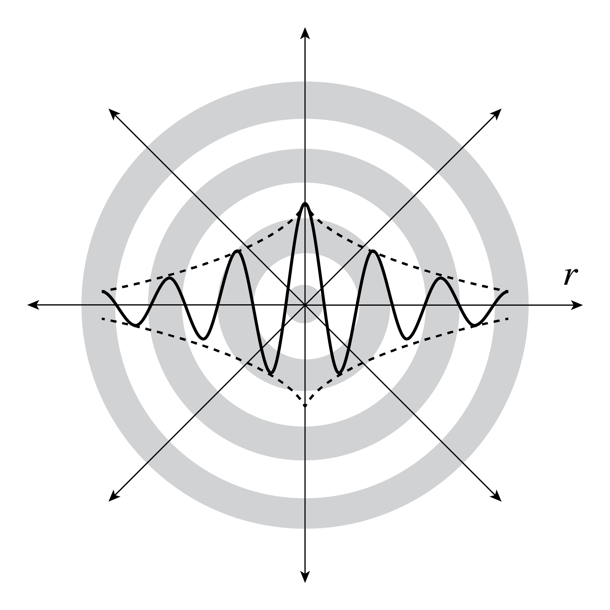
Fig. 3 Spherical wave fronts with amplitude decreasing with distance.

The amplitude of the wave \({\cal A}/r\) is proportional to the inverse distance to the source of sink. Since the time average of the local flux of energy is proportional to the square \({\cal A}^2/r^2\), the time averaged total flux through the surface of any sphere with centre the origin is independent of the radius of the sphere.

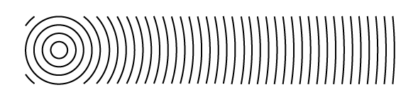
Fig. 4 Planes of constant phase in cross-section. For an observer at large distance to the source the spherical wave looks similar to a plane wave.

Since there is a source or a sink at the origin, (48) satisfies (46) only outside of the origin. There is a \(\delta\)-function as source density on the right-hand side:

(51)\[\begin{align*} \epsilon \mu_0 \frac{\partial^2 }{\partial t^2}{\cal U}(r,t)- \mathbf{\nabla}^2 {\cal U}(r,t)= 4\pi {\cal A}\, \delta(r), \end{align*}\]

where the right-hand side corresponds to either a source or sink at the origin, depending on the sign chosen in the phase.

Using complex notation we have for the outwards propagating wave:

(52)\[\begin{align*} {\cal U}(r,t) =\text{Re}\left[U(\mathbf{r})e^{-i\omega t}\right]= \text{Re}\left[ \frac{A}{r} e^{i ( kr - i\omega t)}\right] \end{align*}\]

with \( U(\mathbf{r})=A \exp( ikr)/r\) and \(A={\cal A}\exp(i\varphi)\), where \(\varphi\) is the argument and \({\cal A}\) is the modulus of the complex number \(A\).

In Fig. 3 and Fig. 4 spherical wave fronts are shown. For an observer who is at a large distance from the source, the spherical wave looks like a plane wave which propagates from the source towards the observer (or in the opposite direction, if there is a sink).

Time-Harmonic Maxwell Equations in Matter

We now return to the Maxwell equations and consider time-harmonic electromagnetic fields, because these are by far the most important fields in optics. Using complex notation we have

(53)\[\begin{align*} \mathbf{\mathcal{E}}(\mathbf{r},t) = \text{Re}\left[ \mathbf{E}(\mathbf{r}) e^{-i\omega t}\right], \end{align*}\]

with

(54)\[\begin{split}\begin{align*} E_x(\mathbf{r}) &= | E_x(\mathbf{r}) | e^{i \varphi_x(\mathbf{r})}, \\ E_y(\mathbf{r}) &= | E_y(\mathbf{r}) | e^{i \varphi_y(\mathbf{r})}, \\ E_z(\mathbf{r}) &= | E_z(\mathbf{r}) | e^{i \varphi_z(\mathbf{r})}, \end{align*}\end{split}\]

where \(\varphi_x(\mathbf{r})\) is the argument of the complex number \(E_x(\mathbf{r})\) etc. With similar notations for the magnetic field, we obtain by substitution into Maxwell’s equations (18), (19), (20) and (21), the time-harmonic Maxwell equations for the complex fields:

(55)\[\begin{align*} \mathbf{\nabla} \times \mathbf{E} & = i\omega \mu_0 \mathbf{H}, & \text{Faraday's Law}, \end{align*}\]

(56)\[\begin{split}\begin{align*} \\ \mathbf{\nabla} \times \mathbf{H} & = -i\omega \epsilon\mathbf{E} + \sigma \mathbf{E} + \mathbf{J}_{ext}, & \text{Maxwell's Law}, \end{align*}\end{split}\]

(57)\[\begin{split}\begin{align*} \\ \mathbf{\nabla} \cdot \epsilon \mathbf{E} & = \varrho_{ext}, & \text{Gauss's Law}, \end{align*}\end{split}\]

(58)\[\begin{split}\begin{align*} \\ \mathbf{\nabla} \cdot \mathbf{H} & = 0, & \text{no magnetic charge},\end{align*}\end{split}\]

where the time derivative has been replaced by multiplication of the complex fields by \(-i\omega\).

In the time-harmonic Maxwell equations, the conductivity is sometimes included in the imaginary part of the permittivity:

(59)\[\begin{align*} \epsilon = \epsilon_0\left[ 1 + \chi_e + i \frac{\sigma}{\omega} \right]. \end{align*}\]

Although it is convenient to do this in Maxwell’s Law (56), one should remember that in Gauss’s Law (57), the original permittivity: \(\epsilon=1+\chi_e\) should still be used. When there are no external sources: \(\varrho_{ext}=0\) and the material is homogeneous (i.e. \(\chi_e\) and \(\sigma\) are independent of position), then (57) is equivalent to

(60)\[\begin{align*} \mathbf{\nabla} \cdot \mathbf{E} =0. \end{align*}\]

Hence in this (important) special case, (59) for the permittivity can safely be used without the risk of confusion.

We see that when we use (59), the conductivity makes the permittivity complex and dependent on frequency. But actually, also for insulators (\(\sigma=0\)), the permittivity \(\epsilon\) depends in general on frequency and is complex with a positive imaginary part. The positive imaginary part of \(\epsilon\) is a measure of the absorption of the light by the material. The property that the permittivity depends on the frequency is called dispersion. Except close to a resonance frequency, the imaginary part of \(\epsilon(\omega)\) is small and the real part is a slowly increasing function of frequency. This is called normal dispersion. This is illustrated with the refractive index of different glass shown in Fig. 5

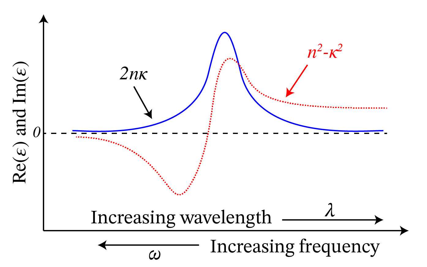
Fig. 5 Real part \(n^2-\kappa^2\) and imaginary part \(2n\kappa\) of the permittivity \(\epsilon=(n+i\kappa)^2\), as function of wavelength and of frequency near a resonance.

Near a resonance, the real part is rapidly changing and decreases with \(\omega\) (this behaviour is called anomalous dispersion), while the imaginary part has a maximum at the resonance frequency of the material, corresponding to maximum absorption at a resonance as seen in Fig. 6. At optical frequencies, mostly normal dispersion occurs and for small-frequency bands such as in laser light, it is often sufficiently accurate to use the value of the permittivity and the conductivity at the centre frequency of the band.

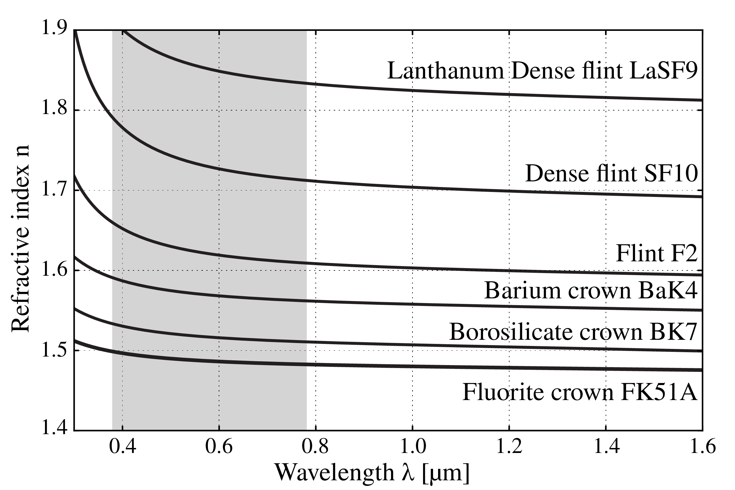
Fig. 6 Refractive index as function of wavelength for several types of glass (from Wikimedia Commons by Geek3 / CC BY-SA).

In many books the following notation is used: \(\epsilon=(n+i \kappa)^2\), where \(n\) and \(\kappa\) (“kappa”, not to be confused with the wave number \(k\)) are both real and positive, with \(n\) the refractive index and \(\kappa\) a measure of the absorption. We then have \(\text{Re}(\epsilon)=n^2-\kappa^2\) and \(\text{Im}(\epsilon)=2 n \kappa\) (see Fig. 5). Note that although \(n\) and \(\kappa\) are both positive, \(\text{Re}(\epsilon)\) can be negative for some frequencies. This happens for metals in the visible part of the spectrum.

Remark. When \(\epsilon\) depends on frequency, Maxwell’s equations in the form (19) and (20) for fields that are not time-harmonic can strictly speaking not be valid, because it is not clear which value of \(\epsilon\) corresponding to which frequency should be chosen. In fact, in the case of strong dispersion, the products \(\epsilon \mathbf{\mathcal{E}}\) should be replaced by convolutions in the time domain. Since we will almost always consider fields with a narrow-frequency band, we shall not elaborate on this issue further.

Time-Harmonic Electromagnetic Plane Waves

In this section we assume that the material in which the wave propagates has conductivity which vanishes: \(\sigma=0\), does not absorb the light and is homogeneous, i.e. that the permittivity \(\epsilon\) is a real constant. Furthermore, we assume that in the region of space of interest there are no sources. These assumptions imply in particular that (60) holds. The electric field of a time-harmonic plane wave is given by

(61)\[\begin{align*} \mathbf{\mathcal{E}}(\mathbf{r},t) = \text{Re}\left[ \mathbf{E}(\mathbf{r}) e^{-i \omega t}\right], \end{align*}\]

with

(62)\[\begin{align*} \mathbf{E}(\mathbf{r})= \mathbf{A} e^{i \mathbf{k}\cdot \mathbf{r}}, \end{align*}\]

where \(\mathbf{A}\) is a constant complex vector (i.e. it is independent of position and time):

(63)\[\begin{align*} \mathbf{A} = A_x \hat{\mathbf{x}} + A_y \hat{\mathbf{y}} + A_z \hat{\mathbf{z}}, \end{align*}\]

with \(A_x=|A_x| e^{i \varphi_x}\) etc… The wave vector \( \mathbf{k}\) satisfies (38). Substitution of (62) into (60) implies that

(64)\[\begin{align*} \mathbf{E}(\mathbf{r})\cdot \mathbf{k} =0, \end{align*}\]

for all \(\mathbf{r}\) and hence (61) implies that also the physical real electric field is in every point \(\mathbf{r}\) perpendicular to the wave vector: \(\mathbf{\mathcal{E}}(\mathbf{r},t)\cdot \mathbf{k}=0\). For simplicity we now choose the wave vector in the direction of the \(z\)-axis and we assume that the electric field vector is parallel to the \(x\)-axis. This case is called a \(x\)-polarised electromagnetic wave. The complex field is then written as

(65)\[\begin{align*} \mathbf{E}(z) = A e^{i k z} \hat{\mathbf{x}}, \end{align*}\]

where \(k=\omega \sqrt{\epsilon \mu_0}\) and \(A=|A| \exp(i \varphi)\). It follows from Faraday’s Law (55)) that

(66)\[\begin{align*} \mathbf{H}(z) = \frac{k}{\omega \mu_0} \hat{\mathbf{z}}\times \hat{\mathbf{x}} A e^{ik z} = \sqrt{\frac{\epsilon}{ \mu_0}} Ae^{i k z } \hat{\mathbf{y}}. \end{align*}\]

The real electromagnetic field is thus:

(67)\[\begin{align*} \mathbf{\mathcal{E}}(z,t) &= \text{Re}\left[ \mathbf{E}(z)e^{-i\omega t}\right] = |A|\cos(kz -\omega t + \varphi) \hat{\mathbf{x}}, \end{align*}\]

(68)\[\begin{split}\begin{align*} \\ \mathbf{\mathcal{H}}(z,t) &= \text{Re}\left[ \mathbf{H}(z) e^{-i\omega t}\right] = \sqrt{\frac{\epsilon}{ \mu_0}} |A| \cos( k z - \omega t + \varphi) \hat{\mathbf{y}}.\end{align*}\end{split}\]

We conclude that in a lossless medium, the electric and magnetic field of a plane wave are in phase and at every point and at every instant perpendicular to the wave vector and to each other. As illustrated in Fig. 7, at any given time the electric and the magnetic field achieve their maximum and minimum values in the same points.

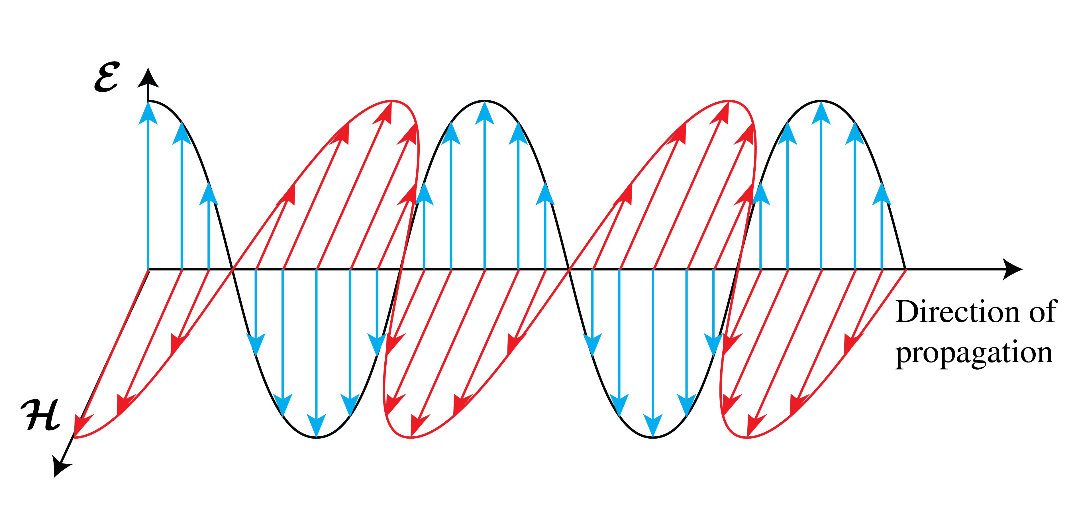
Fig. 7 The time-harmonic vectors \(\mathbf{\mathcal{E}}\) and \(\mathbf{\mathcal{H}}\) of a plane polarised wave are perpendicular to each other and to the direction of the wave vector which is also the direction of \(\mathbf{\mathcal{E}}\times \mathbf{\mathcal{H}}\).

Field of an Electric Dipole

An other important solution of Maxwell’s equation is the field radiated by a time-harmonic electric dipole, i.e. two opposite charges with equal strength that move time-harmonically around their centre of mass. In this section the medium is homogeneous, but it may absorb part of the light, i.e. the permittivity may have a nonzero imaginary part. An electric dipole is the classical electromagnetic model for an atom or molecule. Because the optical wavelength is much larger than an atom and molecule, these charges may be considered to be concentrated both in the same point \(\mathbf{r}_0\). The charge and current densities of such an elementary dipole are

(69)\[\begin{align*} \rho &= -\mathbf{p} \cdot \mathbf{\nabla} \delta(\mathbf{r}-\mathbf{r}_0), \end{align*}\]

(70)\[\begin{split}\begin{align*} \\ \mathbf{J} &= -i\omega \mathbf{p} \delta(\mathbf{r}-\mathbf{r}_0),\end{align*}\end{split}\]

with \(\mathbf{p}\) the dipole vector, defined by

(71)\[\begin{align*} \mathbf{p}= q \mathbf{a}, \end{align*}\]

where \(q>0\) is the positive charge and \(\mathbf{a}\) is the position vector of the positive with respect to the negative charge.

The field radiated by an electric dipole is very important. It is the fundamental solution of Maxwell’s equations, in the sense that the field radiated by an arbitrary distribution of sources can always be written as a superposition of the fields of elementary electric dipoles. This follows from the fact that Maxwell’s equations are linear and any current distribution can be written as a superposition of elementary dipole currents.

The field radiated by an elementary dipole in \(\mathbf{r}_0\) in homogeneous matter can be computed analytically and is given by^[4]

(72)\[\begin{align*} \mathbf{E}(\mathbf{r}) &= \left\{ k^2 \hat{\mathbf{ R}} \times \left(\mathbf{p} \times \hat{\mathbf{R}} \right) + \left( 3 \hat{\mathbf{R}} \cdot \mathbf{p}\, \hat{\mathbf{R}} - \mathbf{p} \right) \left( \frac{1}{R^2}-\frac{ik}{R}\right) \right\} \frac{e^{i k R}}{4 \pi \epsilon R}, \end{align*}\]

(73)\[\begin{split}\begin{align*} \\ \mathbf{H}(\mathbf{r}) &= \frac{k^2 c}{n} \left( 1 + \frac{i}{kR} \right)\, \hat{\mathbf{R}} \times \mathbf{p} \frac{e^{i k R}}{4 \pi R},\end{align*}\end{split}\]

where \(k=k_0 n \), with \(k_0\) bthe wave number in vacuum and \(n=\sqrt{\epsilon/\epsilon_0}\), and with \(\mathbf{R}=\mathbf{r}-\mathbf{r}_0\), \(\hat{\mathbf{R}}=\mathbf{R}/R\). It is seen that the complex electric and magnetic fields are proportional to the complex spherical wave:

\[ \frac{e^{i k R}}{R}\]

discussed in Time-Harmonic Spherical Waves, but that these fields contain additional position dependent factors. In particular, at large distance to the dipole:

(74)\[\begin{align*} \mathbf{H}(\mathbf{r}) & \approx & \frac{k^2 c}{n} \hat{\mathbf{R}} \times **p** \frac{e^{i k R}}{4 \pi R}, \end{align*}\]

(75)\[\begin{split}\begin{align*} \\ \mathbf{E}(\mathbf{r}) & \approx & k^2 \hat{\mathbf{R}} \times \left( \mathbf{p} \times \hat{\mathbf{R}} \right) \frac{e^{i k R}}{4 \pi \epsilon R} = - \sqrt{\frac{\mu_0}{\epsilon}} \hat{\mathbf{R}} \times \mathbf{H}(\mathbf{r}).\end{align*}\end{split}\]

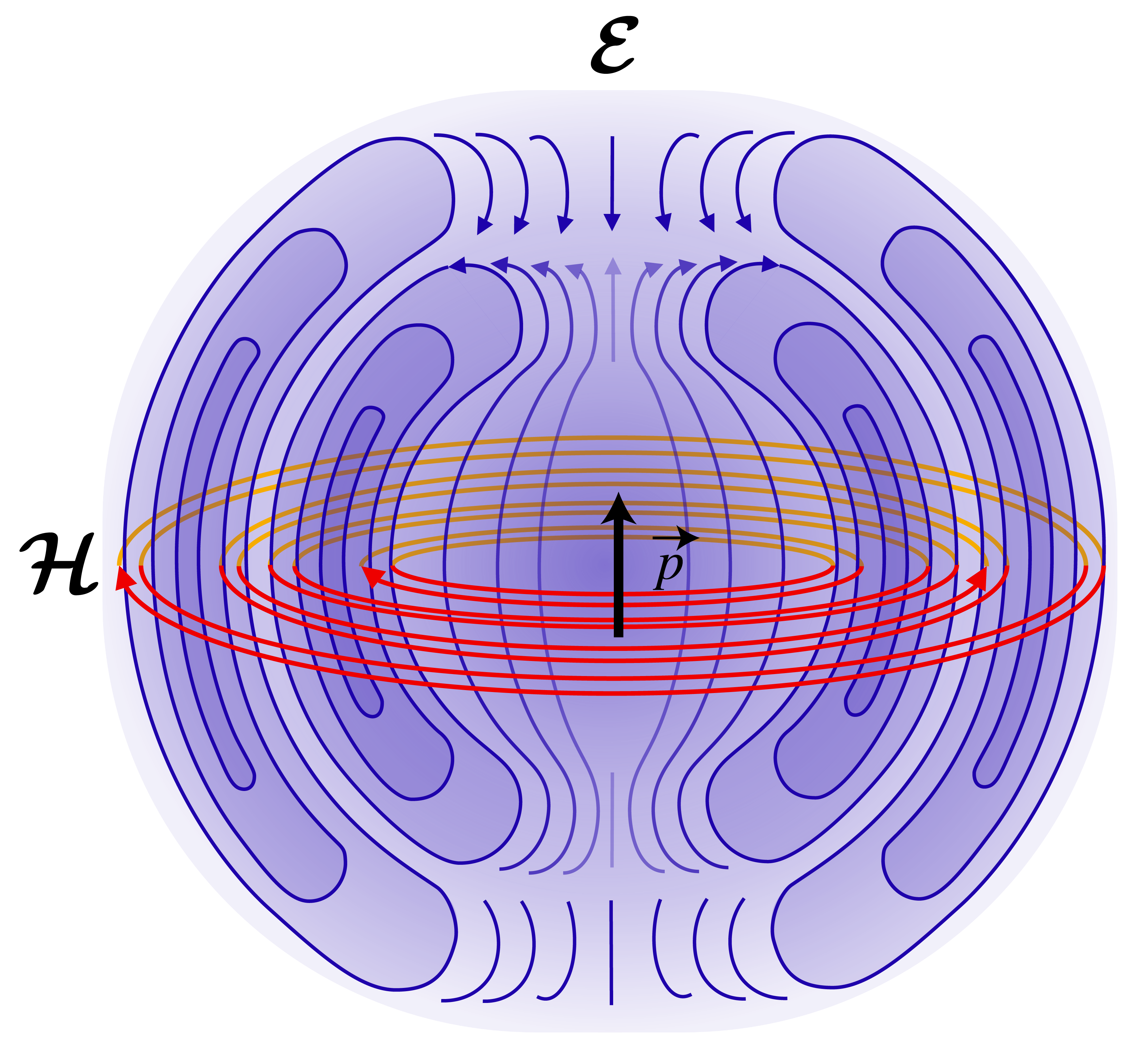
Fig. 8 Electric and magnetic field lines created by a radiating dipole (from Wikimedia Commons, original JPG due to Averse, SVG by Maschen. / CC0).

In Fig. 8 are drawn the electric and magnetic field lines of a radiating dipole. For an observer at large distance from the dipole, the electric and magnetic fields are perpendicular to each other and perpendicular to the direction of the line of sight \(\hat{\mathbf{R}}\) from the dipole to the observer. Furthermore, the electric field is in the plane through the dipole vector \(\mathbf{p}\) and the vector \(\hat{\mathbf{R}}\), while the magnetic field is perpendicular to this plane. So, for a distant observer the dipole field is similar to that of a plane wave which propagates from the dipole towards the observer and has an electric field parallel to the plane through the dipole and the line of sight \(\hat{\mathbf{R}}\) and perpendicular to \(\hat{\mathbf{R}}\). Furthermore, the amplitudes of the electric and magnetic fields depend on the direction of the line of sight, with the field vanishing when the line of sight \(\hat{\mathbf{R}}\) is parallel to the dipole vector \(\mathbf{p}\) and with maximum amplitude when \(\hat{\mathbf{R}}\) is in the plane perpendicular to the dipole vector. This result agrees with the well-known radiation pattern of an antenna when the current of the dipole is in the same direction as that of the antenna.

Electromagnetic Energy

The total energy stored in the electromagnetic field per unit of volume at a point \(\mathbf{r}\) is equal to the sum of the electric and the magnetic energy densities. We postulate that the results for the energy densities derived in electrostatics and magnetostatics are also valid for the fast-oscillating fields in optics; hence we assume that the total electromagnetic energy density is given by:

(76)\[\begin{align*} U_{em} (\mathbf{r},t)=\frac{\epsilon}{2} \mathbf{\mathcal{E}}(\mathbf{r},t)\cdot \mathbf{\mathcal{E}}(\mathbf{r},t) + \frac{\mu_0}{2} \mathbf{\mathcal{H}}(\mathbf{r},t)\cdot \mathbf{\mathcal{H}}(\mathbf{r},t). \end{align*}\]

It is to be noticed that we assume in this section that the permittivity is real, i.e. there is no absorption and the permittivity does not include the conductivity.

Time dependent electromagnetic fields propagate energy. The flow of electromagnetic energy at a certain position \(\mathbf{r}\) and time \(t\) is given by the Poynting vector, which is defined by

(77)\[\begin{align*} \mathbf{\mathcal{S}}(\mathbf{r},t) = \mathbf{\mathcal{E}}(\mathbf{r},t)\times \mathbf{\mathcal{H}}(\mathbf{r},t). \end{align*}\]

More precisely, the flow of electromagnetic energy through a small surface \(\mathrm{d}S \) with normal \(\hat{\mathbf{n}}\) at point \(\mathbf{r}\) is given by

(78)\[\begin{align*} \mathbf{\mathcal{S}}(\mathbf{r},t) \cdot \hat{\mathbf{n}} \mathrm{d}S. \end{align*}\]

If this scalar product is positive, the energy flow is in the direction of \(\hat{\mathbf{n}}\), otherwise it is in the direction of \(-\hat{\mathbf{n}}\). Hence the direction of the vector \(\mathbf{\mathcal{S}}(\mathbf{r},t)\) is the direction of the flow of energy at point \(\mathbf{r}\) and the length \(\| \mathbf{\mathcal{S}}(\mathbf{r},t)\|\) is the amount of the flow of energy, per unit of time and per unit of area perpendicular to the direction of \(\mathbf{\mathcal{S}}\). This quantity has unit J/(s,\(\text{m}^2\)).

That the Poynting vector gives the flow of energy can be seen in a dielectric for which dispersion may be neglected by the following derivation. We consider the change with time of the total electromagnetic energy in a volume \(V\):

(79)\[\begin{align*} \frac{d}{d t } \int\!\int\!\int_V U_{em}(\mathbf{r},t) \, \mathrm{d}V = \int\!\int\!\int_V \epsilon\frac{\partial \mathbf{\mathcal{E}}(\mathbf{r},t)}{\partial t} \cdot \mathbf{\mathcal{E}}(\mathbf{r},t) + \mu_0 \frac{\partial \mathbf{\mathcal{H}}(\mathbf{r},t)}{\partial t} \cdot \mathbf{\mathcal{H}}(\mathbf{r},t) \mathrm{d}V. \end{align*}\]

By substituting (18), (19) and using

(80)\[\begin{align*} -\mathbf{\mathcal{A}}\cdot \mathbf{\nabla} \times \mathbf{\mathcal{B}} +\mathbf{\mathcal{B}}\cdot \mathbf{\nabla} \times \mathbf{\mathcal{A}} = \mathbf{\nabla} \cdot (\mathbf{\mathcal{A}}\times \mathbf{\mathcal{B}}), \end{align*}\]

which holds for any two vector fields, we find

(81)\[\begin{split}\begin{align*} \int\!\int\!\int_V \epsilon \mathbf{\mathcal{E}}(\mathbf{r},t)\cdot \frac{\partial}{\partial t} \mathbf{\mathcal{E}}(\mathbf{r},t) + \mu_0 \mathbf{\mathcal{H}}(\mathbf{r},t)\cdot \frac{\partial}{\partial t} \mathbf{\mathcal{H}}(\mathbf{r},t) \mathrm{d}V \\ = \int\!\int\!\int_V \mathbf{\mathcal{E}}(\mathbf{r},t)\cdot \mathbf{\nabla} \times \mathbf{\mathcal{H}}(\mathbf{r},t) - \mathbf{\mathcal{H}}(\mathbf{r},t)\cdot \mathbf{\nabla} \times \mathbf{\mathcal{E}}(\mathbf{r},t) \mathrm{d}V - \int\!\int\!\int_V \sigma \mathbf{\mathcal{E}}(\mathbf{r},t) \cdot \mathbf{\mathcal{E}}(\mathbf{r},t) \mathrm{d}V \\ - \int\!\int\!\int_V \mathbf{\mathcal{E}}(\mathbf{r},t) \cdot \mathbf{\mathcal{J}}_{ext}(\mathbf{r},t) \mathrm{d}V \\ = -\int\!\int\!\int_V \mathbf{\nabla} \cdot (\mathbf{\mathcal{E}}\times \mathbf{\mathcal{H}}) \mathrm{d}V - \int\!\int\!\int_V \sigma \mathbf{\mathcal{E}}(\mathbf{r},t) \cdot \mathbf{\mathcal{E}}(\mathbf{r},t) \mathrm{d}V - \int\!\int\!\int_V \mathbf{\mathcal{E}}(\mathbf{r},t) \cdot \mathbf{\mathcal{J}}_{ext}(\mathbf{r},t) \mathrm{d}V \\ = - \int\!\int_S (\mathbf{\mathcal{E}}\times \mathbf{\mathcal{H}})\cdot \hat{\mathbf{n}} \mathrm{d}S - \int\!\int\!\int_V \sigma \mathbf{\mathcal{E}}(\mathbf{r},t) \cdot \mathbf{\mathcal{E}}(\mathbf{r},t) \mathrm{d}V- \int\!\int\!\int_V \mathbf{\mathcal{E}}(\mathbf{r},t) \cdot \mathbf{\mathcal{J}}_{ext}(\mathbf{r},t) \mathrm{d}V, \\ \end{align*}\end{split}\]

where \(S\) is the surface bounding volume \(V\) and \(\hat{\mathbf{n}}\) is the unit normal on \(S\) pointing out of \(V\). Hence,

(82)\[\begin{split}\begin{align*} \frac{d}{d t } \int\!\int\!\int_V U_{em}(\mathbf{r},t) \, \mathrm{d}V+ \int\!\int\!\int_V \sigma \mathbf{\mathcal{E}}(\mathbf{r},t) \cdot \mathbf{\mathcal{E}}(\mathbf{r},t) \mathrm{d}V+ \int\!\int\!\int_V \mathbf{\mathcal{E}}(\mathbf{r},t) \cdot \mathbf{\mathcal{J}}(\mathbf{r},t) \mathrm{d}V \\ = -\int\!\int_S \mathbf{\mathcal{S}}(\mathbf{r},t) \cdot \hat{\mathbf{n}} \mathrm{d}S. \end{align*}\end{split}\]

This equation says that the rate of change with time of the electromagnetic energy in a volume \(V\) plus the work done by the field on the conduction and external currents inside \(V\) is equal to the influx of electromagnetic energy through the boundary of \(V\).

Remark. The energy flux \(\mathbf{\mathcal{S}}\) and the energy density \(U_{em}\) depend quadratically on the field. For \(U_{em}\) the quadratic dependence on the electric and magnetic fields is clear. To see that the Poynting vector is also quadratic in the electromagnetic field, one should realise that the electric and magnetic fields are inseparable: they together form the electromagnetic field. Stated differently: if the amplitude of the electric field is doubled, then also that of the magnetic field is doubled and hence the Poynting vector is increased by the factor 4. Therefore, when computing the Poynting vector or the electromagnetic energy density of a time-harmonic electromagnetic field, the real-valued vector fields should be used, i.e. the complex fields should NOT be used. An exception is the calculation of the long-time average of the Poynting vector or the energy density. As we will show in the next section, the time averages of the energy flux and energy density of time-harmonic fields can actually be expressed quite conveniently in terms of the complex field amplitudes.

If we subsitute the real fields (65), (66) of the plane wave in the Poynting vector and the electromagnetic energy density we get:

(83)\[\begin{align*} \mathbf{\mathcal{S}}(z,t) = \mathbf{\mathcal{E}}(z,t)\times \mathbf{\mathcal{H}}(z,t) = \sqrt{\frac{\epsilon}{ \mu_0}} |A|^2 \cos^2(k z -\omega t + \varphi)\, \hat{\mathbf{z}}, \end{align*}\]

(84)\[\begin{align*} U_{em} (z,t) = \epsilon |A|^2 \cos^2(k z - \omega t+\varphi). \end{align*}\]

We see that the energy flow of a plane wave is in the direction of the wave vector, which is also the direction of the phase velocity. Furthermore, it changes with time at frequency \(2\omega\).

Time-Averaged Energy of Time-Harmonic Fields

Optical frequencies are in the range of \(5 \times 10^{14}\) Hz and the fastest detectors working at optical frequencies have integration times larger than \(10^{-10}\) s. Hence there is no detector which can measure the time fluctuations of the electromagnetic fields at optical frequencies and any detector always measures an average value, taken over an interval of time that is very large compared to the period \(2\pi/\omega\) of the light wave, typically at least a factor \(10^5\) longer. We therefore compute averages over such time intervals of the Poynting vector and of the electromagnetic energy. Because the Poynting vector and energy density depend nonlinearly (quadratically) on the field amplitudes, we can not perform the computations using the complex amplitudes and take the real part afterwards, but have instead to start from the real quantities. Nevertheless, it turns out that the final result can be conveniently expressed in terms of the complex field amplitudes.

Consider two time-harmonic functions:

(85)\[\begin{align*} {\cal A}(t)&= \text{Re}\left[ A e^{-i\omega t}\right]= |A| \cos ( \varphi_A -\omega t) \end{align*}\]

(86)\[\begin{split}\begin{align*} \\ {\cal B}(t) &= \text{Re}\left[ B e^{-i\omega t}\right] = |B| \cos(\varphi_B-\omega t),\end{align*}\end{split}\]

with \(A=|A| \exp(i\varphi_A)\) and \(B=|B| \exp(i\varphi_B)\) the complex amplitudes. For a general function of time \(f(t)\) we define the time average over an interval T at a certain time \(t\), by

(87)\[\begin{align*} \frac{1}{T} \int_{t-T/2}^{t+T/2} f(t') \text{d} t'. \end{align*}\]

where \(T\) is much larger (say a factor of \(10^5\)) than the period of the light. It is obvious that for time-harmonic fields the average does not depend on the precise time \(t\) at which it is computed. and we therefore take \(t=0\) and write

(88)\[\boxed{\begin{align*} \braket{ f(t) } = \lim_{T\rightarrow \infty} \frac{1}{T} \int_{-T/2}^{T/2} f(t) \text{d} t. \end{align*}}\]

With

\[\begin{align*} {\cal A}(t)= \text{Re}\left[ A e^{-i\omega t}\right] = \frac{1}{2} \left[A e^{-i\omega t} + A^* e^{i \omega t}\right], \end{align*}\]

where \(A^*\) is the complex conjugate of \(A\), and with a similar expression for \({\cal B}(t)\), it follows that

(89)\[\begin{split}\begin{align*} \lim_{T\rightarrow \infty} \frac{1}{T} \int_{-T/2}^{T/2} {\cal A}(t) {\cal B}(t) \mathrm{d}t &= \lim_{T\rightarrow \infty}\frac{1}{4T} \int_{-T/2}^{T/2} \left[ A B^* + A^* B + A B e^{-2i\omega t} + A^* B^* e^{2i\omega t}\right] \mathrm{d}t \\ &= \lim_{T\rightarrow \infty} \frac{1}{4} \left[ AB^* + A^* B + A B \frac{ e^{i \omega T}- e^{-i \omega T} }{2 iT \omega} + A^* B^* \frac{ e^{i \omega T}-e^{-i \omega T} }{2 iT \omega} \right] \\ &= \frac{1}{2} \text{Re} \left[ A B^* \right], \end{align*}\end{split}\]

This important result will be used over and over again. In words:

Note

The average of the product of two time-harmonic quantities over a long time interval compared with the period, is half the real part of the product of the complex amplitude of one quantity and the complex conjugate of the other.

If we apply this to Poynting’s vector of a general time-harmonic electromagnetic field:

\[\begin{split}\begin{align*} \mathbf{\mathcal{E}}(\mathbf{r},t) &= \text{Re}\left[ \mathbf{E}(\mathbf{r}) e^{-i\omega t}\right], \\ \mathbf{\mathcal{H}}(\mathbf{r},t) &= \text{Re}\left[ \mathbf{H}(\mathbf{r}) e^{-i\omega t}\right], \end{align*}\end{split}\]

then we find that the time-averaged energy flow denoted by \(\mathbf{S}(\mathbf{r})\) is given by

(90)\[\begin{align*} \mathbf{S}(\mathbf{r}) = \lim_{T\rightarrow \infty} \frac{1}{T} \int_{-T/2}^{T/2} \mathbf{\mathcal{S}}(\mathbf{r},t) dt = \frac{1}{2} \text{Re}\left[ \mathbf{E} \times \mathbf{H}^* \right]. \end{align*}\]

Similarly, the time-averaged electromagnetic energy density is:

(91)\[\begin{split}\begin{align*} <U_{en}(\mathbf{r})> &\stackrel{\text{def}}{=} & \lim_{T\rightarrow \infty}\frac{1}{T} \int_{-T/2}^{T/2} U_{en}(\mathbf{r}, t) \mathrm{d}t = \frac{1}{2} \epsilon \mathbf{E}(\mathbf{r})\cdot \mathbf{E}(\mathbf{r})^* + \frac{\mu_0}{2} \mathbf{H}(\mathbf{r})\cdot \mathbf{H}(\mathbf{r})^* \\ &= \frac{1}{2} \epsilon |\mathbf{E}(\mathbf{r})|^2 + \frac{\mu_0}{2} |\mathbf{H}(\mathbf{r})|^2. \end{align*}\end{split}\]

For the special case of plane wave (65), (66) in a medium without absorption, we get:

(92)\[\begin{align*} \mathbf{S} = \frac{1}{2} \sqrt{\frac{\epsilon}{ \mu_0}} \text{Re}\left[ A A^*\right]\hat{\mathbf{z}} = \frac{1}{2}\sqrt{\frac{\epsilon}{ \mu_0}} |A|^2 \hat{\mathbf{z}}. \end{align*}\]

The length of vector (92) is the time-averaged flow of energy per unit of area in the direction of the plane wave and is commonly called the intensity of the wave. For the time-averaged electromagnetic energy density of the plane wave, we get:

(93)\[\begin{align*} <U_{en}> = \frac{1}{2} \epsilon |A|^2 + \frac{1}{2\mu_0}\mu_0 \epsilon |A|^2 = \epsilon |A|^2. \end{align*}\]

Note

For a plane wave both the time-averaged energy flux and the time-averaged energy density are proportional to the squared modulus of the complex electric field.

Reflection and Transmission at an Interface

When an electromagnetic field is incident on an interface between different media, the field is partially reflected and partially transmitted. An important special case is that of a monochromatic plane wave which is incident on a planar interface as in Fig. 10.

Let the interface be the plane \(z=0\) between materials in \(z<0\) and \(z>0\) with permittivities \(\epsilon_i\) and \(\epsilon_t\), respectively. We first assume that the materials are lossless, i.e. that the permittivities are real. The plane wave is incident from medium \(z<0\) and the incident electromagnetic field is given by:

(94)\[\begin{align*} \mathbf{\mathcal{E}}^{i}(\mathbf{r},t) &= \text{Re}\left[ \mathbf{E}^i(\mathbf{r})e^{-i\omega t}\right]= \text{Re}\left[ \mathbf{A}^i e^{i (\mathbf{k}^i\cdot \mathbf{r} -\omega t)} \right], \end{align*}\]

(95)\[\begin{split}\begin{align*} \\ \mathbf{\mathcal{H}}^i(\mathbf{r},t) &= \text{Re}\left[ \mathbf{H}^i(\mathbf{r}) e^{-i\omega t}\right] = \text{Re} \left[ \frac{\mathbf{k}^i}{\omega \mu_0} \times \mathbf{A}^i e^{i (\mathbf{k}^i\cdot \mathbf{r} -\omega t)} \right],\end{align*}\end{split}\]

where \(\mathbf{k}^i= k_x^i \hat{\mathbf{x}} +k_y^i\hat{\mathbf{y}} + k_z^i \hat{\mathbf{z}}\), with

(96)\[\begin{align*} k_z^i=\sqrt{k_0^2 \epsilon_i- (k_x^i)^2- (k_y^i)^2}. \end{align*}\]

Because the time dependence is given by \(\exp(-i\omega t)\) with \(\omega>0\) and the incident wave propagates in the positive \(z\)-direction, the positive square root is chosen for \(k_z^i\). Part of the incident field is reflected into \(z<0\) and part is transmitted into \(z>0\). The reflected field is written as

(97)\[\begin{align*} \mathbf{\mathcal{E}}^{r}(\mathbf{r},t) &= \text{Re}\left[ \mathbf{E}^r(\mathbf{r})e^{-i\omega t}\right]= \text{Re}\left[ \mathbf{A}^r e^{i (\mathbf{k}^r \cdot \mathbf{r} -\omega t)}\right], \end{align*}\]

(98)\[\begin{split}\begin{align*} \\ \mathbf{\mathcal{H}}^{r}(\mathbf{r},t) &= \text{Re}\left[ \mathbf{H}^r(\mathbf{r})e^{-i\omega t}\right]= \text{Re}\left[ \frac{\mathbf{k}^r}{\omega \mu_0}\times \mathbf{A}^r e^{i (\mathbf{k}^r \cdot \mathbf{r} -\omega t)}\right],\end{align*}\end{split}\]

where \(\mathbf{k}^r= k_x^r \hat{\mathbf{x}} +k_y^r\hat{\mathbf{y}} + k_z^r \hat{\mathbf{z}} \), with

(99)\[\begin{align*} k_z^r=-\sqrt{k_0^2 \epsilon_i- (k_x^r)^2-(k_y^r)^2}, \end{align*}\]

where the minus sign is chosen because the reflected wave propagates in the negative \(z\)-direction. The transmitted field is for \(z>0\)

(100)\[\begin{align*} \mathbf{\mathcal{E}}^{t}(\mathbf{r},t) &= \text{Re}\left[ \mathbf{E}^t(\mathbf{r})e^{-i\omega t}\right]= \text{Re}\left[ \mathbf{A}^t e^{i (\mathbf{k}^t\cdot \mathbf{r} -\omega t)} \right],. \end{align*}\]

(101)\[\begin{split}\begin{align*} \\ \mathbf{\mathcal{H}}^{t}(\mathbf{r},t) &= \text{Re}\left[ \mathbf{H}^t(\mathbf{r})e^{-i\omega t}\right]= \text{Re}\left[ \frac{\mathbf{k}^t}{\omega\mu_0}\times \mathbf{A}^t e^{i (\mathbf{k}^t\cdot \mathbf{r} -\omega t)} \right],\end{align*}\end{split}\]

where \(\mathbf{k}^t= k_x^t \hat{\mathbf{x}} +k_y^t \hat{\mathbf{y}} + k_z^t \hat{\mathbf{z}}\), with

(102)\[\begin{align*} k_z^t=\sqrt{k_0^2 \epsilon_t- (k_x^t)^2-(k_y^t)^2}. \end{align*}\]

Our aim is to determine \(\mathbf{A}^r\) and \(\mathbf{A}^t\) for given \(\mathbf{A}^i\).

There exist conditions for the continuity of the tangential and the normal components of both the electric and magnetic fields at an interface between different media. The boundary conditions for the tangential components follow from the Maxwell equations that contain the curl-operator, i.e. (55) and (56). There holds for the interface \(z=0\) with the incident, reflected and transmitted plane waves introduced above:

(103)\[\begin{align*} \hat{\mathbf{z}} \times (\mathbf{E}^i + \mathbf{E}^r)=\hat{\mathbf{z}} \times \mathbf{E}^t, \end{align*}\]

(104)\[\begin{split}\begin{align*} \\ \hat{\mathbf{z}} \times (\mathbf{H}^i + \mathbf{H}^r)=\hat{\mathbf{z}} \times \mathbf{H}^t,\end{align*}\end{split}\]

where \(\hat{\mathbf{z}}\) is the unit normal on the interface. This means that the tangential components of the total electric and total magnetic field are continuous across the interface, or explicitly:

(105)\[\begin{align*} E_x^i(x,y,0) + E_x^r(x,y,0) &= E_x^t(x,y,0), \end{align*}\]

(106)\[\begin{split}\begin{align*} \\ E_y^i(x,y,0) + E_y^r(x,y,0) &= E_y^t(x,y,0),\end{align*}\end{split}\]

and similarly for the magnetic field.

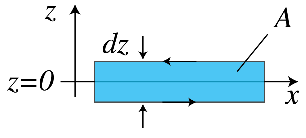
Fig. 9 Closed loop in the \((x,z)\)-plane enclosing the area \(A\) and surrounding part of the interface \(z=0\), as used in Stokes’ Law to derive the continuity of the electric and magnetic components which are tangential to the interface and parallel to the plane through the loop.

We will only demonstrate that the tangential components of the electric field are continuous. By choosing a closed loop in the \((x,z)\)-plane which is intersected by the interface \(z=0\) as shown in Fig. 9, and integrating the \(y\)-component of Faraday’s Law (18) for the total electromagnetic field over the area \(A\) bounded by the loop \({\cal L}\), we obtain:

(107)\[\begin{split}\begin{align*} -\mu_0 \frac{d}{dt} \int\!\int_A \hat{\mathbf{y}} \cdot \mathbf{\mathcal{H}} \mathrm{d}A &= \int\!\int_A \hat{\mathbf{y}} \cdot \mathbf{\nabla} \times \mathbf{\mathcal{E}} \mathrm{d}A \\ &= \oint_{\cal L} \mathbf{\mathcal{E}} \cdot \mathrm{d}\mathbf{l}, \end{align*}\end{split}\]

where in the last step we used Stokes’ theorem with the direction of integration over the loop given by that of the direction of rotation of a screw driver when it moves in the direction of the normal \(\hat{\mathbf{y}}\). In words: the rate of change of the magnetic flux through the surface \(A\) is equal to the integral of the tangential electric field over the bounding closed loop \({\cal L}\).

By taking the limit \(\mathrm{d}z\rightarrow 0\), the surface integral and the integrals over the vertical parts of the loop vanish and there remain only the integrals of the tangential electric field over the horizontal parts parallel to the \(x\)-axis of the loop on both sides of the interface \(z=0\). Since these integrals are traversed in opposite directions and the lengths of these parts are the same and arbitrary, we conclude for the loop as shown in Fig. 9 that

(108)\[\begin{align*} \lim_{z\uparrow 0} \mathbf{\mathcal{E}}_x(x,y,z,t) = \lim_{z\downarrow 0} \mathbf{\mathcal{E}}_x(x,y,z,t), \end{align*}\]

where \(\mathbf{\mathcal{E}}\) is the total electric field, i.e. it is equal to the sum of the incident and the reflected field for \(z<0\), and equal to the transmitted field in \(z>0\). By choosing the closed loop in the \((y,z)\)-plane instead of the \((x,z)\)-plane one finds similarly that the \(y\)-component of the electric field is continuous. The continuity of the tangential components of the magnetic field are derived in a similar manner.

Our derivation holds for electromagnetic fields of arbitrary time dependence. Furthermore, the derivation used above for the planar interface \(z=0\) can easily be generalized for curved surfaces. Therefore we conclude:

Note

The tangential electric and magnetic field components are continuous across any interface.

By integrating Maxwell’s equations that contain the div-operator (20), (21) over a pill box with height \(\mathrm{d}z\) and top and bottom surfaces on either side and parallel to the interface, and considering the limit \(\mathrm{d}z\rightarrow 0\), we find continuity relations for the normal components of the fields:

(109)\[\begin{align*} \lim_{z\uparrow 0} \epsilon_i \hat{\mathbf{z}} \cdot\mathbf{\mathcal{E}}(x,y,z,t) &= \lim_{z\downarrow 0} \epsilon_t \hat{\mathbf{z}} \cdot \mathbf{\mathcal{E}}(x,y,z,t), \end{align*}\]

(110)\[\begin{align*} \lim_{z\uparrow 0} \hat{\mathbf{z}} \cdot\mathbf{\mathcal{H}}(x,y,z,t) &= \lim_{z\downarrow 0} \hat{\mathbf{z}}\cdot \mathbf{\mathcal{H}}(x,y,z,t),\end{align*}\]

Note

The normal components of \(\epsilon \mathbf{\mathcal{E}}\) and \(\mathbf{\mathcal{H}}\) are continuous across an interface.

Remarks.

• Since the derived boundary conditions hold for all times t, it follows that for time-harmonic fields they also hold for the complex fields. Hence (103) and (104) hold and similarly we find that the normal components of \(\epsilon \mathbf{E}\) and \(\mathbf{H}\) are continuous.

• When the magnetic permeability is discontinuous, we have that the normal component of \(\mu \mathbf{\mathcal{H}}\) is continuous across the interface. But as has been remarked before, at optical frequencies the magnetic permeability is often that of vacuum and we assume this to be the case throughout this book.

Snell’s Law

By substituting the complex electric fields derived from (94), (97) and (100) into equation (103), we get

(111)\[\begin{align*} \hat{\mathbf{z}}\times \left[ \mathbf{A}^i e^{i (k_x^i x + k_y^i y)} + \mathbf{A}^r e^{i (k_x^r x + k_y^r y)}\right] = \hat{\mathbf{z}}\times \mathbf{A}^t e^{i (k_x^t x + k_y^t y)}, \end{align*}\]

Since this equation must be satisfied for all points \((x,y)\), it follows that

(112)\[\begin{align*} k_x^i = k_x^r=k_x^t, \end{align*}\]

(113)\[\begin{split}\begin{align*} \\ k_y^i = k_y^r=k_y^t.\end{align*}\end{split}\]

Hence, the tangential components of the wave vectors of the incident, reflected and transmitted waves are identical. In fact, if (112) would not hold, then by keeping \(y\) fixed, the exponential functions in (111) would not all have the same periodicity as functions of \(x\) and then (111) could never be satisfied for all \(x\). The same argument with \(x\) kept fixed leads to the conclusion (113).

Without restricting the generality, we will from now on assume that the coordinate system is chosen such that

(114)\[\begin{align*} k_y^i=k_y^r=k_y^t=0. \end{align*}\]

The plane through the incident wave vector and the normal to the interface is called the plane of incidence. Hence in the case of (114) the plane of incidence is the \((x,z)\)-plane.

Since the length of the wave vectors \(\mathbf{k}^i\) and \(\mathbf{k}^r\) is \(k_0 n_i\), with \(k_0\) the wave number in vacuum and \(n_i=\sqrt{\epsilon_i/\epsilon_0}\) the refractive index, and since the length of \(\mathbf{k}^t\) is \(k_0n_t\), with \(n_t=\sqrt{\epsilon_t/\epsilon_0}\), it follows from (112)

(115)\[\begin{align*} \sin \theta_i = \frac{k_x^i}{k_0 n_i}= \frac{k_x^r}{k_0 n_i}=\sin \theta_r, \end{align*}\]

and

(116)\[\begin{align*} n_i \sin \theta_i = \frac{k_x^i}{k_0} = \frac{k_x^t}{k_0} = n_t \sin \theta_t, \end{align*}\]

where the angles are as in Fig. 10. Hence,

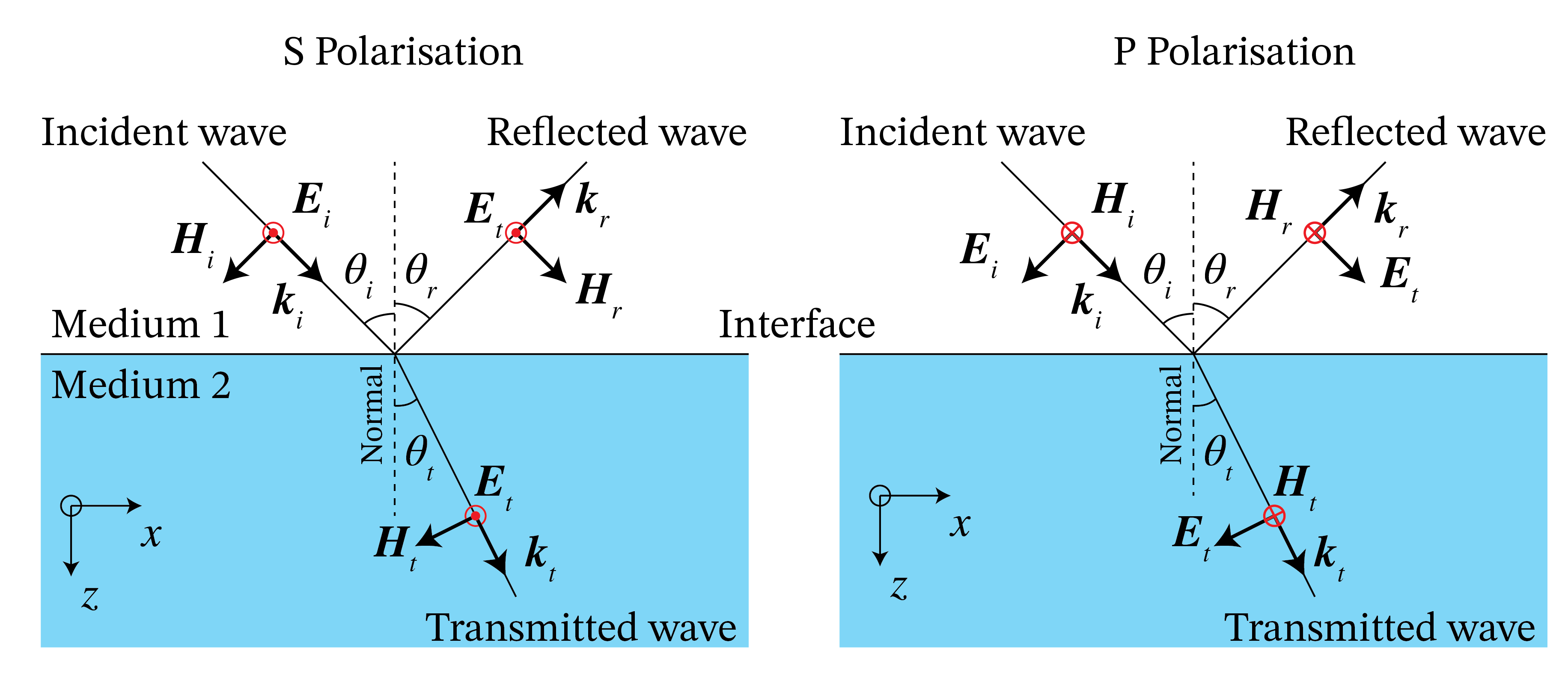
Fig. 10 The incident, reflected, and transmitted wave vectors with the electric and magnetic vectors for s- and p-polarisation. For s-polarisation the electric field points out of the plane at the instant shown while for p-polarisation the magnetic field points out of the plane at the instant shown.

(117)\[\boxed{\begin{align*} \theta_i &= \theta_r,\hspace{1cm}\;\text{angle of reflection = angle of incidence}, \end{align*}}\]

(118)\[\begin{split}\boxed{\begin{align*} \\ n_i \sin \theta_i &= n_t \sin \theta_t, \;\;\; \text{ Snell's Law}. \end{align*}}\end{split}\]

Snell’s Law^[5] implies that when the angle of incidence \(\theta_i\) increases, the angle of transmission increases as well. If the medium in \(z<0\) is air with refractive index \(n_i=1\) and the other medium is glass with refractive index \(n_t=1.5\), then the maximum angle of transmission occurs when \(\theta_i=90^o\) with

(119)\[\begin{align*} \theta_{t,max} = \arcsin(n_i/n_t)=41.8^o. \end{align*}\]

In case the light is incident from glass, i.e. \(n_i=1.5\) and \(n_t=1.0\), the angle of incidence \(\theta_i\) cannot be larger than \(41.8^o\) because otherwise there is no real solution for \(\theta_t\). It turns out that when \(\theta_i> 41.8^o\), the wave is totally reflected and there is no propagating transmitted wave in air. As explained in Total Internal Reflection and Evanescent Waves, this does however not mean that there is no field in \(z>0\). In fact there is a non-propagating so-called evanescent wave in \(z>0\). The angle \(\theta_{i,crit}=41.8^o\) is called the critical angle of total internal reflection. It exists only if a wave is incident from a medium with larger refractive index on a medium with lower refractive index (\(n_t<n_i\)). The critical angle is independent of the polarisation of the incident wave.

Fresnel Coefficients

Because of (112) and (114), we write \(k_x=k_x^i=k_x^r=k_x^t\) and therefore \(k_z^i = \sqrt{k_0^2\epsilon_i - k_x^2} = -k_z^r\) and \(k_z^t=\sqrt{k_0^2\epsilon_t-k_x^2}\). Hence,

(120)\[\begin{align*} \mathbf{k}^i = k_x \hat{\mathbf{x}} + k_z^i \hat{\mathbf{z}}, \;\;\; \mathbf{k}^r = k_x\hat{\mathbf{x}} - k_z^i \hat{\mathbf{z}}, \end{align*}\]

and

(121)\[\begin{align*} \mathbf{k}^t = k_x \hat{\mathbf{x}} + k_z^t \hat{\mathbf{z}}. \end{align*}\]

According to (64), for the incident, reflected and transmitted plane waves there must hold:

(122)\[\begin{align*} \mathbf{A}^i \cdot \mathbf{k}^i = \mathbf{A}^r\cdot \mathbf{k}^r = \mathbf{A}^t\cdot \mathbf{k}^t =0. \end{align*}\]

We choose an orthonormal basis perpendicular to \(\mathbf{k}^i\) with unit vectors:

(123)\[\begin{align*} \hat{\mathbf{s}} = \hat{\mathbf{y}}, \quad \hat{\mathbf{p}}^i = \frac{1}{|\mathbf{k}^i|} \left( -k_z^i \hat{\mathbf{x}}+ k_x \hat{\mathbf{z}}\right), \end{align*}\]

where

(124)\[\begin{align*} |\mathbf{k}^i| = \sqrt{\mathbf{k}^i \cdot (\mathbf{k}^i)^*} = \sqrt{k_x^2 + |k_z^i|^2}, \end{align*}\]

and where in writing the complex conjugate we anticipate the case the \(k_z^i\) is complex, which may happen for example when \(\epsilon_i\) is complex (a case that has been excluded so far but which later will be considered) or in the case of evanescent waves discussed in Total Internal Reflection and Evanescent Waves. Note that when \(k_z^i\) is real, \(|\mathbf{k}^i|=\sqrt{k_x^2 + (k_z^i)^2}=k_0n_i\). It is easy to see that the basis (123) is orthonormal in the space of two-dimensional complex vectors and that \(\hat{\mathbf{s}}\cdot\mathbf{k}^i=\hat{\mathbf{p}}^i\cdot \mathbf{k}^i=0\). The vector \(\hat{\mathbf{s}}\) is perpendicular to the plane of incidence, therefore the electric field component in this direction is polarised perpendicular to the plane of incidence and is called s-polarised (“Senkrecht” in German). The other basis vector \(\hat{\mathbf{p}}^i\) is (for real \(\mathbf{k}^i\)) parallel to the plane of incidence and when the electric component in this direction it is called p-polarised. The complex vector \(\mathbf{A}^i\) can be expanded on this basis:

(125)\[\begin{align*} \mathbf{A}^i= A^i_s \, \hat{\mathbf{y}} + A^i_p \, \hat{\mathbf{p}}^i. \end{align*}\]

Since

(126)\[\begin{align*} \mathbf{k}^i\times \hat{\mathbf{y}}= |\mathbf{k}^i| \hat{\mathbf{p}}^i, \;\;\; \mathbf{k}^i \times \hat{\mathbf{p}}^i= - \frac{k_0^2 \epsilon_i}{|\mathbf{k}^i|} \hat{\mathbf{y}}, \end{align*}\]

it follows that the electric and magnetic field of the incident plane wave can be written as

(127)\[\begin{align*} \mathbf{E}^i(\mathbf{r}) &= \left(A^i_s\, \hat{\mathbf{y}} + A^i_p \, \hat{\mathbf{p}}^i\right) e^{i\mathbf{k}^i\cdot \mathbf{r}}, \end{align*}\]

(128)\[\begin{split}\begin{align*} \\ \mathbf{H}^i(\mathbf{r}) &=\left( \frac{ |\mathbf{k}^i| }{\omega \mu_0} A^i_s \, \hat{\mathbf{p}}^i - \frac{ \omega \epsilon_0\epsilon_i}{|\mathbf{k}^i|} A^i_p \, \hat{\mathbf{y}} \right) e^{i\mathbf{k}^i\cdot \mathbf{r}}.\end{align*}\end{split}\]

The reflected field is expanded on the basis \(\hat{\mathbf{y}}\) and \(\hat{\mathbf{p}}^r\) with

(129)\[\begin{align*} \hat{\mathbf{p}}^r = -\frac{1}{|\mathbf{k}^i|} \left( k_z^i \hat{\mathbf{x}} + k_x \hat{\mathbf{z}}\right). \end{align*}\]

The sign in front of the unit vector \(\hat{\mathbf{p}}^r\) is chosen such that that its \(x\)-component is the same as that of \(\hat{\mathbf{p}}^i\). Since

(130)\[\begin{align*} \mathbf{k}^r\times \hat{\mathbf{y}}= -|\mathbf{k}^i| \hat{\mathbf{p}}^r, \;\;\; \mathbf{k}^r \times \hat{\mathbf{p}}^r= \frac{k_0^2 \epsilon_i}{|\mathbf{k}^i|} \hat{\mathbf{y}}, \end{align*}\]

it follows that

(131)\[\begin{align*} \mathbf{E}^r(\mathbf{r}) &= \left(A^r_s\, \hat{\mathbf{y}} + A^r_p \, \hat{\mathbf{p}}^r \right) e^{i\mathbf{k}^r\cdot \mathbf{r}}, \end{align*}\]

(132)\[\begin{split}\begin{align*} \\ \mathbf{H}^r(\mathbf{r}) &=\left( -\frac{|\mathbf{k}^i|}{\omega \mu_0} A^r_s \, \hat{\mathbf{p}}^r + \frac{ \omega\epsilon_0 \epsilon_i}{|\mathbf{k}^i|} A^r_p \, \hat{\mathbf{y}} \right) e^{i\mathbf{k}^r\cdot \mathbf{r}},\end{align*}\end{split}\]

where we used that \(\mathbf{k}^r\cdot \mathbf{k}^r=k_0^2 n_i^2 \) and \(|\mathbf{k}^r|=\sqrt{k_x^2 + |k_z^r|^2}=\sqrt{k_x^2+|k_z^i|^2}=|\mathbf{k}^i|\). For the transmitted plane wave we use the basis \(\hat{\mathbf{y}}\) and \(\hat{\mathbf{p}}^t\) with

(133)\[\begin{align*} \hat{\mathbf{p}}^t= \frac{1}{|\mathbf{k}^t|} \left( -k_z^t \hat{\mathbf{x}}+ k_x \hat{\mathbf{z}}\right), \end{align*}\]

where \(\hat{\mathbf{p}}^t\) is chosen such that the \(x\)-component of \(\hat{\mathbf{p}}^t\) has the same sign as the \(x\)-component of \(\hat{\mathbf{p}}^i\). Since

(134)\[\begin{align*} \mathbf{k}^t\times \hat{\mathbf{y}}= |\mathbf{k}^t| \hat{\mathbf{p}}^t, \;\;\; \mathbf{k}^t \times \hat{\mathbf{p}}^t= - \frac{k_0^2 \epsilon_t}{|\mathbf{k}^t|} \hat{\mathbf{y}}, \end{align*}\]

we get

(135)\[\begin{align*} \mathbf{E}^t(\mathbf{r}) &= \left( A^t_s\, \hat{\mathbf{y}} + A^t_p \, \hat{\mathbf{p}}^t \right) e^{i\mathbf{k}^t\cdot \mathbf{r}}, \end{align*}\]

(136)\[\begin{split}\begin{align*} \\ \mathbf{H}^t(\mathbf{r}) &= \left( \frac{ |\mathbf{k}^t|}{\omega \mu_0} A^t_s \, \hat{\mathbf{p}}^t - \frac{ \omega \epsilon_0\epsilon_t}{|\mathbf{k}^t|} A^t_p \, \hat{\mathbf{y}} \right) e^{i\mathbf{k}^t\cdot \mathbf{r}},\end{align*}\end{split}\]

We now consider an s-polarised incident plane wave, i.e. \(A^i_p=0\). We will show that all boundary conditions can be satisfied by \(A^r_p=A^t_p=0\) and by appropriately expressing \(A^r_s\) and \(A^t_s\) in terms of \(A^i_s\). This implies that if the incident plane wave is s-polarised, the reflected and transmitted waves are s-polarised as well. For s-polarisation, the electric field has only a \(y\)-component and this component is tangential to the interface \(z=0\). This leads to the condition

(137)\[\begin{align*} A_s^i + A^r_s = A^t_s. \end{align*}\]

The only tangential component of the magnetic field is the \(x\)-component and requiring it to be continuous for \(z=0\) leads to

(138)\[\begin{align*} -k_z^i A_s^i + k_z^i A^r_s = -k_z^t A^t_s. \end{align*}\]

Solving (137), (138) for \(A_s^r\) and \(A^t_s\) gives the following formula for the reflection and transmission coefficients:

(139)\[\boxed{\begin{align*} r_s & = \frac{A^r_s}{A^i_s} = \frac{k_z^i-k_z^t}{k_z^i + k_z^t}, \end{align*}}\]

(140)\[\begin{split}\boxed{\begin{align*} \\ t_s & = \frac{A^t_s}{A^i_s} = \frac{2k_z^i}{k_z^i + k_z^t}. \end{align*}}\end{split}\]

Only the magnetic field has a \(z\)-component and it easy to verify that \(H^i_z + H^r_z = H_z\) for \(z=0\).

By looking at the case of a p-polarised incident wave: \(A^i_s=0\), we see that the expression for the magnetic field in the p-polarised case become similar (except for the chosen signs) to that of the electric field for s-polarisation and conversely. Enforcing the continuity of the tangential components at \(z=0\) gives for p-polarisation:

(141)\[\boxed{\begin{align*} r_p & = \frac{A^r_p}{A^i_p} = - \frac{\frac{k_z^i}{\epsilon_i}-\frac{k_z^t}{\epsilon_t}}{\frac{k_z^i}{\epsilon_i} + \frac{k_z^t}{\epsilon_t}}, \end{align*}}\]

(142)\[\begin{split}\boxed{\begin{align*} \\ t_p & = \frac{A^t_p}{A^i_p} =\frac{\epsilon_i |\mathbf{k}^t|}{\epsilon_t|\mathbf{k}^i|} \frac{\frac{2 k_z^i}{\epsilon_i}}{\frac{k_z^i}{\epsilon_i} + \frac{k_z^t}{\epsilon_t}}. \end{align*}}\end{split}\]

It is easy to verify that \(E_z\) is the only normal component and that \(\epsilon_i (E^i_z+E^r_z)=\epsilon_t E^t_z\) for \(z=0\).

The reflection and transmission coefficients \(r_s\), \(r_p\), \(t_s\) and \(t_p\) are called Fresnel coefficients. As follows from the derivation, there is no cross talk between s- and p-polarised plane waves incident on a planar interface. A generally polarised incident plane wave can always be written as a linear combination of s- and a p-polarised incident plane waves. Because in general \(r_s\neq r_p\) and \(t_s\neq t_p\), it follows that the reflected and transmitted fields are also linear combinations of s- and p-polarised fields, but with different coefficients (weights) of these two fundamental polarisation states than for the incident wave.

Remarks.

• In the derivation of the Fresnel coefficients the continuity of the normal field components was not used and was automatically satisfied. The reason is that the electromagnetic fields of the plane waves where chosen to be perpendicular to the wave vectors. This implies that the divergence of \(\epsilon \mathbf{\mathcal{E}}\) and of \(\mathbf{\mathcal{H}}\) vanishes which in turns implies that the normal components are automatically continuous across the the interface.

• When \(k_z^i\) and \(k_z^t\) are both real, we have \(|\mathbf{k}^i|=k_0n_i\) and \(|\mathbf{k}^t|=k_0n_t\) and the Fresnel coefficients can be expressed in the angles \(\theta_i\), \(\theta_r\) and \(\theta_t\) and the refractive indices \(n_i=\sqrt{\epsilon_i}/\epsilon_0\) and \(n_t=\sqrt{\epsilon_t/\epsilon_0}\). Because \(k^i_z=k_0n_i \cos\theta_i\) and \(k^t_z=k_0 n_t \cos \theta_t\), we find

(143)\[\begin{align*} r_s &= \frac{n_i \cos \theta_i-n_t \cos \theta_t}{n_i \cos \theta_i + n_t \cos \theta_t} = -\frac{\sin(\theta_i-\theta_t)}{\sin(\theta_i+\theta_t)}, \end{align*}\]

(144)\[\begin{split}\begin{align*} \\ t_s &= \frac{2 n_i \cos \theta_i }{ n_i \cos \theta_i + n_t \cos \theta_t} = \frac{2 \cos \theta_i \sin \theta_t}{\sin(\theta_i+\theta_t)},\end{align*}\end{split}\]

and

(145)\[\begin{align*} r_p &= - \frac{\frac{\cos\theta_i}{n_i} - \frac{\cos \theta_t}{n_t}}{ \frac{\cos\theta_i}{n_i} + \frac{\cos \theta_t}{n_t}}= -\frac{\tan(\theta_i-\theta_t)}{ \tan(\theta_i+\theta_t)}, \end{align*}\]

(146)\[\begin{split}\begin{align*} \\ t_p &= \frac{\frac{2 \cos\theta_i}{n_i} }{ \frac{\cos\theta_i}{n_i} + \frac{\cos \theta_t}{n_t}}= \frac{ 2 \cos \theta_i \sin\theta_t}{ \sin(\theta_i+\theta_t) \cos(\theta_i-\theta_t)}.\end{align*}\end{split}\]

To obtain the expressions at the far right in (143), (144), (143) and (146) Snell’s Law has been used.

• The advantage of the expressions (139), (140), (141), (142) in terms of the wave vector components \(k_z^i\) and \(k_z^t\) is that these also apply when \(k_z^i\) and/or \(k_z^t\) are complex. The components \(k_z^i\) and/or \(k_z^t\) are complex when there is absorption in \(z<0\) and/or in \(z>0\). When \(\epsilon_i>\epsilon_t\) and the incident angle is above the critical angle, \(k_z^t\) is imaginary (see Total Internal Reflection and Evanescent Waves).

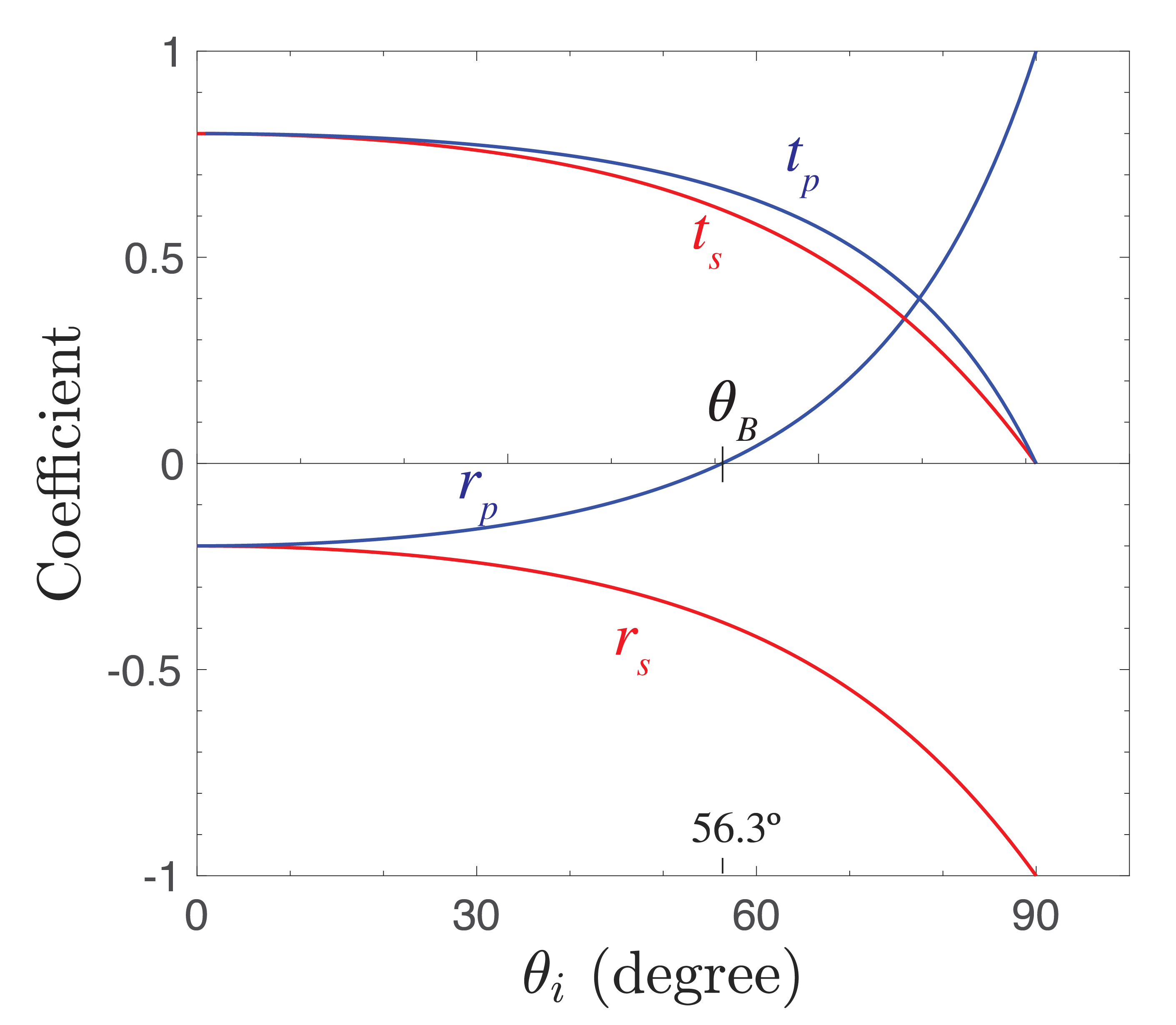
Fig. 11 Reflection and transmission coefficients as function of the angle of incidence of s- and p-polarised waves incident from air to glass. The Brewster angle \(\theta_B\) is indicated.

Properties of the Fresnel Coefficients

For normal incidence: \(\theta_i=0\), Snell’s Law implies: \(\theta_t=0\). Hence, (143), (145) give:

(147)\[\begin{align*} r_s(\theta_i=0) = r_p(\theta_i=0)=\frac{n_i-n_t}{n_i + n_t}, \end{align*}\]

So for normal incidence: \(r_p=r_s\), as expected. Note however that if we would not have defined \(\hat{\mathbf{p}}^r\) such that its tangential components are the same as those of \(\hat{\mathbf{p}}^i\), the two reflection coefficients for normal incidence would have had the opposite signs (as is the case in some books). If the incident medium is air and the other medium is glass (\(n_i=1.0\), \(n_t=1.5\)), we get

(148)\[\begin{align*} r_s(\theta_i=0)=r_p(\theta_i=0)= -0.2, \end{align*}\]

and since the flow of energy is proportional to the square of the field, it follows that 4% of the normal incident light is reflected at the interface between air and glass. Hence a lens of glass without anti-reflection coating reflects approximately 4% of the light at normal incidence. The transmission coefficient for normal incidence is:

(149)\[\begin{align*} t_s(\theta_i=0)=t_p(\theta_i=0)= \frac{2n_i}{n_i+n_t}, \end{align*}\]

which for air-glass becomes \(0.8\).

Remark. Energy conservation requires that the normal component \(<S_z>\) of the time-averaged energy flux through the interface is continuous. By using the formula for the time-averaged Poynting vector of a plane wave (92), it can be verified that the Fresnel coefficients are such that the energy flux is indeed continuous.

It follows from Snell’s Law (118) that when both refractive indices \(n-i\) and \(n_t\) are real, \(\sin \theta_t = (n_i/n_t) \sin \theta_i\). Hence \(\theta_t\) monotonically increases with \(\theta_i\) and therefore there exists some \(\theta_i\) such that

(151)\[\begin{align*} \theta_i + \theta_t = 90^o. \end{align*}\]

For this particular angle of incidence, the denominator of (145) is infinite and hence \(r_p=0\), i.e. the p-polarised wave is not reflected at all. This angle of incidence is called the Brewster angle \(\theta_{B}\)^[6]. It is easy to see from (143) that the reflection is never zero for s-polarisation.

Note

If unpolarised light is incident at the Brewster angle, the reflected light will be purely s-polarised.

Since at the Brewster angle s-polarised light is only partially reflected and the rest is transmitted, the transmitted light at the Brewster angle is a mixture of s- and p-polarisation. We have \(\theta_t=90^o-\theta_i\), hence \(\sin\theta_t=\cos\theta_i\) and by Snell’s Law (writing \(\theta_i=\theta_{B})\):

(151)\[\begin{align*} \tan(\theta_{B})=\frac{n_t}{n_i}. \end{align*}\]

We see that there is always a Brewster angle when both refractive indces are real, independent of whether the wave is incident from the material with the smallest or largest refractive index. For the air-glass interface we have \(\theta_{B}=56.3^o\) and \(\theta_t=33.7^o\). By (143):

(152)\[\begin{align*} r_s(\theta_B=56.3^o)=-0.38, \end{align*}\]

so that \((0.38)^2/2=0.07\), or 7 % of the unpolarised light is reflected as purely s-polarised light at the air glass interface at the Brewster angle. For a wave incident from glass, \(\theta_{B}=33.7^o\).

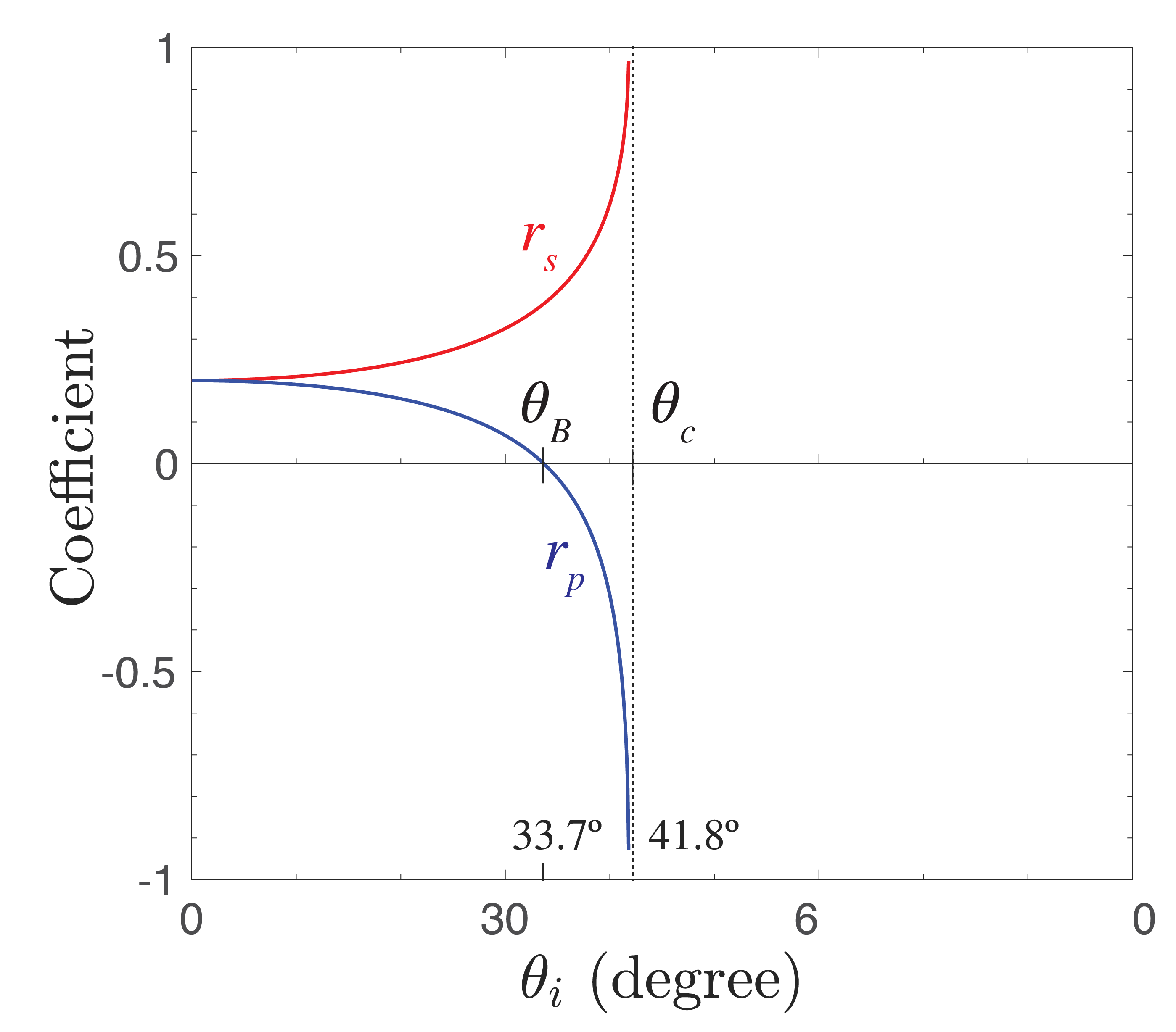
Fig. 12 Reflection and transmission coefficients as function of the angle of incidence of s- and p-polarised waves incident from glass to air.

In Fig. 12 the Fresnel reflection and transmission coefficients of s- and p-polarised waves are shown as functions of the angle of incidence for the case of incidence from air to glass. There is no critical angle of total reflection in this case. The Brewster angle is indicated. It is seen that the reflection coefficients decrease from the values \(-0.2\) for \(\theta_i=0^o\) to -1 for \(\theta_i=90^o\). The transmission coefficients monotonically decrease to \(0\) at \(\theta_i=90^o\).

Fig. 12 shows the Fresnel coefficients when the wave is incident from glass to air. The critical angle is \(\theta_{i,crit}=41.8^o\) as derived earlier. At the angle of total internal reflection the absolute values of the reflection coefficients are identical to 1. There is again an angle where the reflection of p-polarised light is zero \(\theta_{B}=33.7^o\).

Depending on the refractive indices and the angle of incidence, the Fresnel reflection coefficients can be negative. The reflected electric field then has an additional \(\pi\) phase shift compared to the incident wave. In contrast, (provided that the materials are lossless), the transmitted field is always in phase with the incident field, i.e. the transmission coefficients are always positive.

Total Internal Reflection and Evanescent Waves

We return to the case of a wave incident from glass to air, i.e. \(n_i=1.5\) and \(n_t=1\). As has been explained, there is then a critical angle, given by

\[\begin{align*} \sin \theta_{i,crit} = \frac{n_t}{n_i}. \end{align*}\]

This is equivalent to

(153)\[\begin{align*} k_x^{t} = k_0 n_i \sin \theta_{i,crit} = k_0 n_t. \end{align*}\]

The wave vector \(\mathbf{k}^t=k_x^t \hat{\mathbf{x}} + k_z^t\hat{\mathbf{z}}\) in \(z>0\) always satisfies:

(154)\[\begin{align*} (k_x^t)^2 + (k_z^t)^2 = k_0^2 n_t^2, \end{align*}\]

and hence at the critical angle thre holds

(155)\[\begin{align*} k_z^t=0. \end{align*}\]

For angles of incidence above the critical angle we have: \(k_x^t>k_0 n_t \) and it follows from (154) that \((k_z^t)^2=k_0^2n_t^2 -(k_x^t)^2<0\), hence \(k_z^t\) is imaginary:

(156)\[\begin{align*} k_z^t =\pm \sqrt{ k_0^2n_t^2 - (k_x^t)^2} = \pm i \sqrt{(k_x^t)^2-k_0^2}, \end{align*}\]

where the last square root is a positive real number. It can be shown that above the critical angle the reflection coefficients are complex numbers with modulus 1: \(|r_s|=|r_p|=1\). This implies that the reflected intensity is identical to the incident intensity, while at the same time the transmission coefficients are not zero! For example, for s-polarisation we have according to (139), (140):

(157)\[\begin{align*} t_s=1+ r_s \neq 0, \end{align*}\]

because \(r_s \neq -1\) (although \(|r_s|=1\)). Therefore there is an electric field in \(z>0\), given by

(158)\[\begin{align*} \mathbf{E}(x,z)e^{-i \omega t} = t_s e^{i k_x^t x + i k_z^t z -i\omega t} \hat{\mathbf{y}}= t_s e^{i (k_x^t x - \omega t)} e^{ -z \sqrt{(k_x^t)^2-k_0^2n_t^2}} \hat{\mathbf{y}}, \;\; z>0, \end{align*}\]

where we have chosen the \(+\) sign in (156) to prevent the field from blowing up for \(z \rightarrow \infty\). Since \(k_x^t\) is real, the wave propagates in the \(x\)-direction. In the \(z\)-direction, however, the wave is not propagating. Its amplitude decreases exponentially as a function of distance \(z\) to the interface and therefore the wave is confined to a thin layer adjacent to the interface. Such a wave is called an evanescent wave. The Poynting vector of the evanescent wave can be computed and is found to be parallel to the interface. Hence,

Note

The flow of energy of an evanescent wave propagates parallel to the interface, namely in the direction in which \(k_x^t\) is positive.

Hence no energy is transported away from the interface into the air region. We shall return to evanescent waves in the chapter on diffraction theory.

External sources in recommended order

1. Youtube video - 8.03 - Lect 18 - Index of Refraction, Reflection, Fresnel Equations, Brewster Angle - Lecture by Walter Lewin 2. MIT OCW - Reflection at The Air-glass Boundary: demonstration of reflection of polarised light and the Brewster angle.

Fiber Optics

We will show in Scalar Diffraction Optics on diffraction that a light beam ultimately always becomes broader for increasing propagation distance. The divergence means that the energy density in the beam decreases with propagation distance. This divergence can be prevented by letting the light propagate inside a fiber. The guiding of light inside a fiber is based on the phenomenon of total internal reflection. The principle has been known for a long time, but the topic was greatly boosted by the invention of the laser.

Consider a straight glass cylinder of refractive index \(n_2\), surrounded by air with refractive index \(n_1=1<n_2\). The core of the cylinder has a cross section approximately the size of a human hair and hence, although quite small, it is still many optical wavelengths thick. This implies that when light strikes the cylindrical surface, we can locally consider the cylinder as a flat surface. By focusing a laser beam at the entrance plane of the fiber, light can be coupled into the fiber. The part of the light inside the fiber that strikes the cylinder surface at an angle with the normal that is larger than the critical angle of total reflection will be totally reflected. As it hits the opposite side of the cylinder surface, it will again be totally reflected and so on (Fig. 13 top).

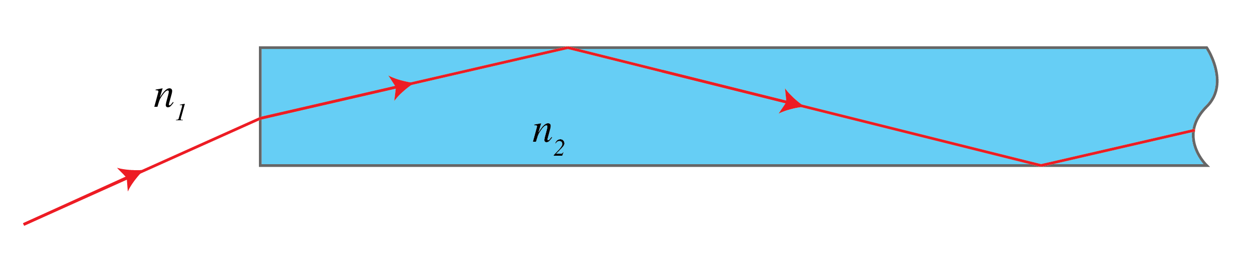
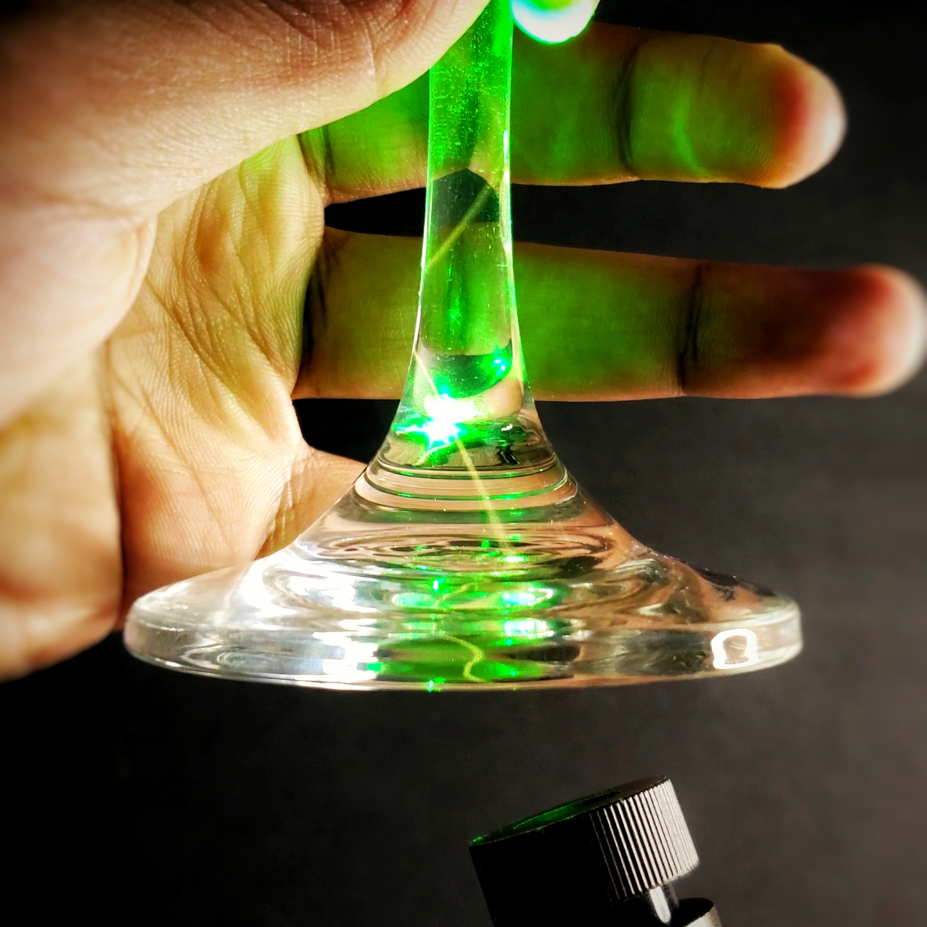
Fig. 13 Top: schematic of a light ray entering a glass fiber; inside the light is totally reflected and is guided by the fiber. middle: Light guided within a piece of glass. (from Wikimedia Commons by Keerthi - CC BY ); bottom: a glass fiber optic image inverter twists an image 180 degrees from its input surface to its output surface.(Image:© SCHOTT)

Since visible light has such high frequencies (order \(10^{15}\) Hz), roughly a hundred thousand times more information can be carried through a fiber than at microwave frequencies. Today fibers with very low losses are fabricated so that signals can be sent around the earth with hardly any attenuation. Abraham van Heel, professor of optics at Delft University of Technology, showed for the first time in a paper published in Nature in 1954^[7] that by packing thousands of fibers into a cable, images can be transferred, even if the bundle is bent (Fig. 13 bottom).

External sources in recommended order

1. MIT OCW - Single Mode Fiber: Demonstration of a single-mode fiber.

2. MIT OCW - Multi-mode Fiber: Demonstration of a multimode fiber.

Khan Academy - Magnetic field created by a current carrying wire (Ampere’s Law)

---

[1]

Units of physical quantities are written between brackets [.].

[2]

Khan Academy - Faraday’s Law Introduction

[3]

[4]

For a derivation see D.J. Griffiths, Introduction to Electrodynamics, Pearson.

[5]

Named after Willebrord Snellius 1580-1626, mathematics professor in Leiden

[6]

MIT OCW - Reflection at The Air-glass Boundary: demonstration of reflection of polarised light and the Brewster angle.

[7]

Van Heel, A. A, New Method of transporting Optical Images without Aberrations. Nature 173, 39 (1954) link