
12. Waves#
In physics a wave is a disturbance or oscillation that travels through space accompanied by a transfer of energy, and may be propagated with little or no net motion of the medium involved. In this section we will consider mechanical waves, in which the particles in a material are oscillating. Examples are the waves in the sea, the wave in the crowd at a stadium, and sound. Later on we will encounter electromagnetic waves in which electric and magnetic fields are oscillating, and which can travel through vacuum. Examples are light and radio signals. In quantum mechanics, we will also encounter what are sometimes referred to as matter waves, where fundamental objects that we usually think of as particles, such as electrons and protons, can also be considered as waves. Finally, recently gravitational waves were discovered, which are vibrations of spacetime itself.
By observing a particle, we know in which direction it moves at any given time. However, as I just stated, the particles in a mechanical wave have no, or almost no, net motion as the wave passes. The wave does have a well-defined direction though: the direction in which energy is transferred. Some waves spread out uniformly, such as a sound wave emanating from a point source. Others are restricted in their motion by the properties of the material they travel in, such as a wave in a string, or by boundary conditions, such as the end of that string. For waves that move (predominantly) in one direction, we can distinguish two fundamental types, illustrated in Fig. 12.1. The first type is the case that the particles oscillate in the same direction as the wave is moving (Fig. 12.1a), which we call a longitudinal wave; sound is an example. The second case is that the particles oscillate in a direction perpendicular to the wave motion, which we call a transverse wave (Fig. 12.1b), of which the waves in a pond are an example.

Fig. 12.1 Two basic types of waves. (a) Longitudinal wave, where the oscillatory motion of the particles is in the same direction as that of the wave. (b) Transverse wave, where the oscillatory motion of the particles is perpendicular to that of the wave.#
12.1. Sinusoidal waves#
Probably the simplest kind of wave is a transverse sinusoidal wave in a one-dimensional string. In such a wave each point of the string undergoes a harmonic oscillation. We will call the displacement from equilibrium \(u\), then we can plot \(u\) as a function of position on the string at a given point in time, Fig. 12.2a, which is a snapshot of the wave. Alternatively, we can plot \(u\) as a function of time for a given point (with given position) on the string, Fig. 12.2b. Because the oscillation is harmonic, the displacement as a function of time is a sine function, with an amplitude (maximum displacement) \(A\) and a period (time between maxima) \(T\).
By definition, each point of the string undergoing a sinusoidal wave undergoes a harmonic oscillation, so for each point we can write \(u(t) = A \cos(\omega t + \phi)\) (equation (8.4)), where as before \(\omega = 2\pi/T\) is the (angular) frequency and \(\phi\) the phase. Two neighboring points on the string are slightly out of phase - if the wave is traveling to the right, then your right-hand neighbor will reach maximum slightly later than you, and thus has a slightly larger phase. The difference in phase is directly proportional to the distance between two points, coming to a full \(2\pi\) (which is of course equivalent to zero) after a distance \(\lambda\), the wavelength. The wavelength is thus the distance between two successive points with the same phase, in particular between two maxima. In between these maxima, the phase runs over the full \(2\pi\), so the wave is also a sinusoid in space, with a ‘spatial frequency’ or wavenumber \(k = 2\pi / \lambda\). Combining the dependencies on space and time in a single expression, we can write for the sinusoidal wave:
The speed of the wave is the distance the wave travels per unit time. A unit time for a wave is one period, as that is the time it takes the oscillation to return to its original point. The distance traveled in one period is one wavelength, as that is the distance between two maxima. The speed is therefore simply their ratio, which can also be expressed in terms of the wave number and frequency:

Fig. 12.2 A sinusoidal transverse wave in space (a) and time (b). The distance between two successive maxima (or any two successive points with equal phase is the wavelength \(\lambda\) of the wave. The maximum displacement is the amplitude \(A\), and the time it takes a single point to go through a full oscillation is the period \(T\).#
12.2. The wave equation#
As with all phenomena in classical mechanics, the motion of the particles in a wave, for instance the masses on springs in Fig. 12.1, are governed by Newton’s laws of motion and the various force laws. In this section we will use these laws to derive an equation of motion for the wave itself, which applies quite generally to wave phenomena. To do so, consider a series of particles of equal mass \(m\) connected by springs of spring constant \(k\), again as in Fig. 12.1a, and assume that at rest the distance between any two masses is \(h\). Let the position of particle \(i\) be \(x\), and \(u\) the distance that particle is away from its rest position; then \(u = x_\mathrm{rest}-x\) is a function of both position \(x\) and time \(t\). Suppose particle \(i\) has moved to the left, then it will feel a restoring force to the right due to two sources: the compressed spring on its left, and the extended spring on its right. The total force to the right is then given by:
Equation (12.3) gives the net force on particle \(i\), which by Newton’s second law of motion (equation (2.5)) equals the particle’s mass times its acceleration. The acceleration is the second time derivative of the position \(x\), but since the equilibrium position is a constant, it is also the second time derivative of the distance from the equilibrium position \(u(x,t)\), and we have:
Equation (12.4) holds for particle \(i\), but just as well for particle \(i+1\), or \(i-10\). We can get an equation for \(N\) particles by simply adding their individual equations, which we can do because these equations are linear. We thus find for a string of particles of length \(L=Nh\) and total mass \(M=Nm\):
Here \(K=k/N\) is the effective spring constant of the \(N\) springs in series. Now take a close look at the fraction on the right hand side of equation (12.5): if we take the limit \(h \to 0\), this is the second derivative of \(u(x,t)\) with respect to \(x\). However, taking \(h\) to zero also takes \(L\) to zero - which we can counteract by simultaneously taking \(N\to\infty\), in such a way that their product \(L\) remains the same. What we end up with is a string of infinitely many particles connected by infinitely many springs - so a continuum of particles and springs, for which the equation of motion is given by the wave equation:
In equation (12.6), \(v_\mathrm{w} = \sqrt{K L^2/M}\) (sometimes also denoted by \(c\)) is the wave speed.
For a wave in a taut string, the one-dimensional description is accurate, and we can relate our quantities \(K\), \(L\) and \(M\) to more familiar properties of the string: its tension \(T=K L\) with the dimension of a force (this is simply Hooke’s law again) and its mass per unit length \(\mu = M/L\), so we get
In two or three dimensions, the spatial derivative in equation (12.6) becomes a Laplacian operator, and the wave equation is given by:
As can be readily seen by writing equation (12.8) in terms of spherical coordinates, if the wave is radial (i.e., only depends on the distance to the source \(r\), and not on the angle), the quantity \(r u(r)\) obeys the one-dimensional wave equation, so we can write down the equation for \(u(r)\) immediately. An important application are sound waves, which spread uniformly in a uniform medium. To find their speed, we characterize the medium in a similar fashion as we did for the string: we take the mass per unit volume, which is simply the density \(\rho\), and the medium’s bulk modulus, which is a measure for the medium’s resistance to compression (i.e., a kind of three-dimensional analog of the spring constant), defined as:
where \(p\) is the pressure (force per unit area) and \(V\) the volume. The bulk modulus is also sometimes denoted as \(K\). The dimensions of the bulk modulus are those of a pressure, or force per unit area, and those of the density are mass per unit volume, so their ratio has the dimension of a speed squared, and the speed of sound is given by:
Equation (12.8) describes a wave characterized by a one-dimensional displacement (either longitudinal or transverse) in three dimensions. In general a wave can have components of both, and the displacement itself becomes a vector quantity, \(\bm{u}(\bm{x}, t)\). In that case the three-dimensional wave equation takes on a more complex form:
where \(\bm{f}\) is the driving force (per unit volume), \(B\) again the bulk modulus, and \(G\) the material’s shear modulus. Equation (12.11) is used for the description of seismic waves in the Earth and the ultrasonic waves with which solid materials are probed for defects.
12.3. Solution of the one-dimensional wave equation#
The one-dimensional wave equation (12.6) has a surprisingly generic solution, due to the fact that it contains second derivatives in both space and time. As you can readily see by inspection, the function \(q(x,t) = x - v_\mathrm{w} t\) is a solution, as is the same function with a plus instead of a minus sign. These functions represent waves traveling to the right (minus) or left (plus) at speed \(v_\mathrm{w}\). However, the shape of the wave does not matter - any function \(F(q) = F(x - v_\mathrm{w} t)\) is a solution of (12.6), as is any function \(G(x + v_\mathrm{w} t)\), and the general solution is the sum of these:
To find a specific solution, we need to look at the initial conditions of the wave, i.e., the conditions at \(t=0\). Because the wave equation is second order in time, we need to specify both the initial displacement and the displacement’s initial velocity, which can be functions of the position. For the most general case we write:
The resulting solution of the one-dimensional wave equation is known as d’Alembert’s equation:
12.4. Wave superposition#
The wave equation (12.6) is linear in the function we’re interested in, the displacement \(u(x,t)\). This simple mathematical statement has important consequences, because it means that if we know any set of solutions, we can create more solutions by making linear combinations of them - so if \(u_1(x,t)\) and \(u_2(x,t)\) are solutions, then so are \(a u_1(x,t) + b u_2(x,t)\) for any choice of \(a\) and \(b\). In physics, this useful property of linear differential equations is known as the principle of superposition. Thanks to this principle, we can study how different waves interact with each other without having to do (much) extra math.
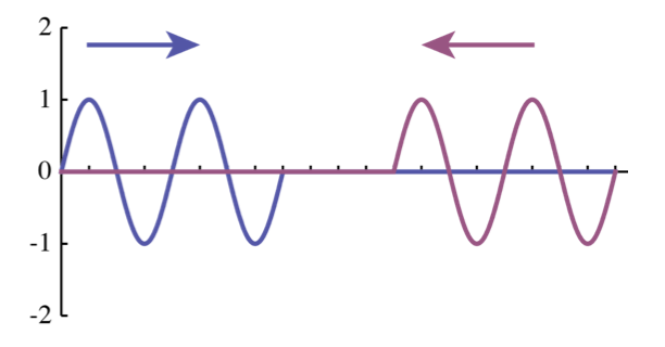
To illustrate, let us consider two one-dimensional waves traveling in opposite directions, Fig. 12.3. As long as the waves do not overlap, the oscillation of any given particle is due to only one wave, and there is no interaction. However, as soon as the waves start overlapping, the oscillations add up, which leads to interference. At some points, the two oscillations will be in phase, resulting in a much larger oscillation amplitude, which we call constructive interference (Fig. 12.3b). At other points, the two oscillations will be out of phase, resulting in a much smaller, or even vanishing oscillation amplitude, which we call destructive interference (Fig. 12.3c). However, the waves themselves remain unaffected, and transmit right through each other, continuing their path as if nothing had happened (Fig. 12.3d).

Fig. 12.3 Two interacting wave packets. The sequence of images shows four snapshots. The blue wave is traveling to the right, the red wave to the left (a). When the waves overlap, the total displacement of the particle is given by the sum of the displacements due to both waves, shown in green. This can lead to both constructive interference (b), when the two waves are in phase, and destructive interference (c), when their phases are opposite. The waves themselves are not affected by the interaction and afterwards travel on as if nothing has happened (d).#
Waves reaching the end of a string, or edge of a pond, or any type of boundary, will not simply disappear. Remember, waves carry energy, and that energy is conserved, so it has to go somewhere once the wave reaches the boundary. If there’s nothing at the boundary, the waves are reflected back into the material. This happens in two cases: a (perfectly) fixed boundary, and a (perfectly) free boundary; in other cases, some of the energy may be transmitted to material on the other side of the boundary (starting a new wave there), whereas the remainder is reflected back into the original material with less energy, resulting in a smaller wave amplitude. A reflected wave travels in the opposite direction to the original wave, so it can interfere with itself. In fact, this interference is a crucial point for being able to meet the boundary conditions. A fixed boundary cannot move, so there must be destructive interference keeping the amplitude there zero at all times - so it follows that a wave reflecting on a fixed boundary undergoes a \(\pi\) phase shift. Free boundaries on the other hand are perfectly free to move, so there is nothing holding it back from reaching the maximal displacement that can be achieved by constructive interference, and the wave reflects without a phase shift.
If you put boundaries on both ends of a string, the wave keeps reflecting back and forth, continuously interfering with itself. To find the resulting shape of the string, we’re going to use the principle of superposition for a simple sinusoidal wave. Let \(u_1(x,t) = A \cos(kx-\omega t)\) be the part of the wave traveling to the right, and \(u_2(x,t) = - A \cos(kx + \omega t)\) be the part traveling to the left. Note the differences: the waves have opposite signs for their speeds, and opposite signs for their displacements, the latter because of the \(\pi\) phase shift (we could also write \(u_2(x,t) = A \cos(kx + \omega t + \pi)\)). The shape of the string is now simply the sum of these two waves:
Equation (12.15) tells us that for a self-interfering wave, the wave no longer moves - instead, each point simply oscillates with frequency \(\omega\) at a position-dependent amplitude \(2 A \sin(kx)\). We call such a wave a standing wave. Standing waves are very common - you’ll get one every time you’ll touch the string of a guitar or violin. Naturally, they are not restricted to one-dimensional systems - the skin of a drum, constrained at the drum’s edge, is put in a standing wave every time someone hits it.
Equation (12.15) describes the shape of a standing wave on a string clamped at both ends. If the string has length \(L\), then by the nature of the boundary conditions, we must have \(u(0,t) = u(L,t) = 0\) for all \(t\). The first condition follows for free (which is of course just due to a good choice of coordinates), but the second puts a constraint on our wave. The displacement can only be zero at all times if the amplitude is identically zero, so we demand that \(\sin(kL) = 0\), or \(L = m \pi /k = m \lambda / 2\), where \(m\) is any positive integer. There are thus infinitely many allowed standing waves, but they are characterized by a discrete number. The allowed waves are known as modes, and the associated number \(m\) is the mode number. The simplest wave, with the lowest possible value, \(m=1\), is known as the fundamental mode. In the fundamental mode, the oscillation of the string has nonzero amplitude everywhere but at the fixed ends; for higher modes, there are also points in between that have zero amplitude, which are known as nodes; points where the amplitude is maximum are sometimes referred to as antinodes.
A discrete spectrum of allowed solutions, characterized by integer numbers, does not only appear in standing mechanical waves, but is also a fundamental aspect of quantum mechanics.

Fig. 12.4 Snapshots of the wave patterns for the first three modes of a standing wave in (a) a string with two clamped ends, (b) a string with one clamped end, or a tube with one closed and one open end, and (c) a tube with two open ends. In each case, the plot shows the amplitude of the standing wave, as a fraction of the amplitude of the traveling wave. At nodes, the amplitude of the standing wave vanishes: destructive interference causes these points to always stand still. At antinodes, the amplitude of the standing wave is maximal, and equals that of the traveling wave. Note that (a) and (b) will occur for transversal waves, whereas (b) and (c) will occur for sound waves. For cases (a) and (c) allowed wavelengths are \(\lambda = 2L / n\), whereas for case (b), allowed wavelengths are \(\lambda = 4L / (2n-1)\).#

12.5. Amplitude modulation#
So far, we’ve mostly considered simple sinusoidal waves with fixed amplitudes. However, the general solution to the wave equation allows for many more interesting wave shapes. An important, and often encountered one is where the wave itself is used as the medium, by changing the amplitude over time:
The wave now consists of two waves: the carrier wave, which travels with the phase velocity \(v_\mathrm{w} = \omega/k\), and the envelope, which travels with the group velocity \(v_\mathrm{g}\). An illustration of a modulated wave is shown in Fig. 12.5. In the common case that the group velocity is independent of the wavelength of the carrier wave, we can rewrite (12.16) to reflect the fact that the amplitude is now also a wave, with speed \(v_\mathrm{g}\):

Fig. 12.5 Amplitude-modulated wave. The amplitude of the carrier wave (blue, traveling at phase velocity \(v_\mathrm{w} = \omega/k\)) is changed over time, resulting in an envelope (red) which travels at the lower group velocity \(v_\mathrm{g}\).#
12.6. Sound waves#
So far, we mostly considered transversal waves, which include waves in strings and waves on the surface of a pond, and are easily visualized. Longitudinal waves, on the other hand, are somewhat harder to draw, but easily heard - as sound is the prime example of a longitudinal wave. Other examples include (some forms of) seismic waves and ultrasound. Many people simply lump all of these together, and use the terms ‘sound waves’ and ‘longitudinal waves’ as synonyms.
We already touched upon the speed of sound waves in Section 12.2 (equation (12.10)). This speed indicates how fast the wavefronts of a sound wave travel; a wavefront is defined as the surface (in three dimensions) where all points have the same phase[1]. To visualize a sound wave we draw a succession of wavefronts one wavelength (or one period) apart. Simple examples include a point source (generating spherical wavefronts) and a planar wave, in which all wave fronts are parallel planes (see Fig. 12.6). The (local) direction of propagation of the wave is the direction perpendicular to the wavefronts, sometimes depicted by a ray.

Fig. 12.6 Snapshots of the wavefronts (points with equal phase) of a longitudinal wave for (a) a point source (with spherical wavefronts) and (b) a planar wave (where all wavefronts are parallel planes). Successive wavefronts are separated by one wavelength.#
Like transversal waves, longitudinal waves exhibit interference, both with other waves they encounter, and by their own reflections. There can therefore be traveling and standing sound waves. Unlike transversal waves on strings however, longitudinal sound waves are typically created in tubes that are open on either one or both ends. A closed end represents a fixed point, just like the fixed end of a string does, resulting in a stringent boundary condition: the interference between the incoming and outgoing wave must be such that the net displacement at the closed end is zero. An open end corresponds to a transversal wave in a string that is not clamped. As the string in that case is free to move, its maximum displacement will equal the amplitude of the wave. In other words, while a closed end corresponds to a node, the open end corresponds to an antinode. For a string (or pipe) with one clamped / closed and one open end, the wavelength of the lowest-order mode (known as the fundamental mode or first harmonic) therefore equals four times the length \(L\) of the string / pipe. The next mode (second harmonic) will have a wavelength of \(4L/3\), and so on (see Fig. 12.4b), resulting in \(\lambda = 4L/(2n-1)\) for the \(n\)th mode. For a tube with two open ends, the fundamental mode is the inverse of that of a string with two clamped ends - so two antinodes at the ends, and a node in the middle (Fig. 12.4c). Like for a clamped string, the allowed wavelengths are therefore \(\lambda = 2L/n\).
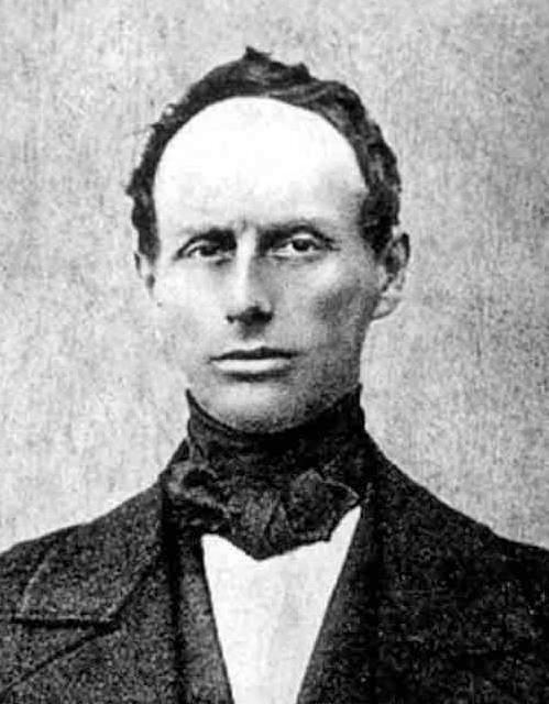
Christian Doppler (1803-1853)
Christian Doppler (1803-1853) was an Austrian physicist. Doppler was a professor of physics at Prague where he developed the notion that the observed frequency of a wave depends on the relative speed of the source and the observer, now known as the Doppler effect. Doppler used this principle to explain the observed colors of binary stars. The principle was developed independently by French physicist Armand Fizeau (1819-1896), and is therefore sometimes referred to as the Doppler-Fizeau effect. In 1847, Doppler moved to Selmecbánya in Hungary, but was forced to leave again soon afterwards due to political unrest in 1848, moving to the university of Vienna. During a visit to Venice in 1853, Doppler died of pulmonary disease, aged only 49.
12.7. The Doppler effect#
The Doppler effect is a physical phenomenon that most people have experienced many times: when a moving source of sound (say an ambulance, or more exactly its siren) is approaching you, its pitch sounds noticeably higher then after it passed you by and is moving away. The effect is due to the fact that the observed wavelength (and therefore frequency / pitch) of sound corresponds to the distance between two points of equal phase (i.e., two sequential wavefronts). Ultimately, the Doppler effect thus originates in a change in reference frame (the same frames we encountered in Section 4.3): what you hear is indeed different from what the ambulance’s driver hears. The latter is easy: the driver isn’t moving with respect to the siren, so (s)he simply hears it at whatever frequency it is emitting. For the stationary observer however, the ambulance moves between emitting the first and second wave crest, and so their distance (and hence the observed wavelength / frequency) changes, see Fig. 12.8.

Fig. 12.8 Doppler effect. The source emits waves with a fixed time interval \(\Delta t\) between successive wavefronts. (a) For observers that are stationary with respect to the source, the distance between wavefronts (in red) is fixed, so they measure the same wavelength as the one emitted by the source. (b) If the source is moving with respect to the observers (here to the right), the observers measure a different distance between arriving wavefronts - compressed (so shorter wavelength / higher frequency) if the source is approaching (green dot), expanded if the source is receding (purple dot).#
Calculating the shift in wavelength is straightforward. Let us call the speed of sound \(v\) and the speed of the source \(u\). The time interval between two wavefronts, as emitted by the source, is \(\Delta t\). In this time interval, the first wavefronts travels a distance \(\Delta s = v \Delta t\), while the source travels a distance \(\Delta x = u \Delta t\). For the observer to which the source is approaching, the actual distance between two emitted wavefronts is thus \(\Delta x' = \Delta s - \Delta x = (v - u) \Delta t\). The actual distance between the wavefronts is the observed wavelength, \(\lambda_\mathrm{obs}\), while the emitted wavelength is \(\lambda = \Delta s = v \Delta t\), so the two are related through
For a source that is moving away, we simply flip the sign of \(u\); naturally for a stationary source we have \(\lambda_\mathrm{obs} = \lambda\). Note that we could also consider a stationary source and a moving observer: the effect would be exactly the same, where in equation (12.18) we define motion towards the source to be the positive direction.
The Doppler effect is usually expressed in terms of frequency instead of wavelength, but that is a trivial step from equation (12.18), as \(f_\mathrm{obs} = v / \lambda_\mathrm{obs}\) and \(f = v / \lambda\), which gives:
Although we discussed the Doppler effect here in the context of sound waves, it occurs for any kind of waves - most notably also light.
Ernst Mach (1838-1916)
Ernst Mach (1838-1916) was an Austrian physicist. Mach was a professor of mathematics and later physics at Graz, Prague and Vienna. His experimental work focused on the properties of waves, especially in light, as well as on the Doppler effect in both light and sound. In 1888, Mach used photography to capture the shock waves created by a supersonic bullet. In addition to physics, Mach was highly interested in philosophy, holding the position that only sensations are real. Consequently, Mach refused to accept that atoms are real, as they could not be observed directly at the time; it was Einstein’s 1905 work on Brownian motion that eventually proved him wrong. The ratio of an object’s speed to the speed of sound is now known as the Mach number in his honor.
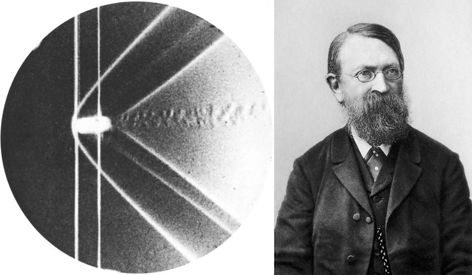
Fig. 12.9 Left: Mach’s picture of the shockwave of a supersonic bullet [3]. Right: Ernst Mach (1902) [4].#
Note that equation (12.18) predicts that the wavelength is zero if the speed of the source equals the speed of the emitted waves. This case is illustrated in Fig. 12.10a, which shows that the wavefronts pile up. For a source moving faster than the wave speed (Fig. 12.10b), the waves follow the source, creating a conical shock wave, with opening angle given by
Both the bow wave of a boat and the sonic boom of a supersonic jet are examples of shock waves.

Fig. 12.10 Shock waves. Like in Fig. 12.8, the source emits wavefronts with a fixed time interval \(\Delta t\). (a) If the source is moving at the same speed as the emitted wave, the wavefronts all collide, creating a shock wave. (b) For a source moving faster than the speed of the waves, the waves all travel behind the source, creating a conical (shock) wave front (as you may have heard after seeing a jet fighter pass overhead). The blue dot indicates the current position of the source, the green dot that one period ago, the red dot two periods ago.#
12.8. Problems#
Exercise 12.1 (Sound waves in a spring)
Sound waves in a spring. In Section 12.2, we found that the speed of a wave in a string is given by \(v = \sqrt{T/\mu}\), with \(T\) the tension in the string and \(\mu\) its mass density (equation (12.7)).
A spring of mass \(m\) and spring constant \(k\) has an unstretched length \(L_0\). Find an expression for the speed of transverse waves on this spring when it’s been stretched to a length \(L\).
You measure the speed of transverse waves in an ideal spring under stretch. You find that at a certain length \(L_1\) it has a value \(v\), and at length \(2L_1\) the wavespeed has value \(3v\). Find an expression for the unstretched length of the spring in terms of \(L_1\).
A uniform cable hangs vertically under its own weight. Show that the speed of waves on the cable is given by \(v = \sqrt{zg}\), where \(z\) is the distance from the bottom of the cable. You may assume that the stretching of the cable is small enough that its mass density can be taken to be uniform.
Show that the time it takes a wave to propagate up the cable in (c) is \(t = 2 \sqrt{L/g}\), with \(L\) the cable length.
Exercise 12.2 (Surface waves on water)
In deep water, the speed of surface waves depends on their wavelength:
Apart from satellite images, offshore storms can also be detected by watching the waves at the beach. Equation (12.21) tells us that the longest-wavelength waves will travel the fastest, so the arrival of such waves, if their amplitude is high, is a foreboding of the possible arrival of a storm (the friction between the wind and the water being the source of the waves). A typical storm may be thus detected from a distance of \(500\;\mathrm{km}\), and travel at \(50\;\mathrm{km}/\mathrm{h}\). Suppose the detected waves have crests \(200\;\mathrm{m}\) apart. Estimate the time interval between the detection of these waves and the arrival of the storm (in the case the storm moves straight towards the beach). In shallow water, the speed of surface waves becomes (to first order) independent of the wavelength, but scales with the depth of the water instead
(12.22)#\[v = \sqrt{gd}.\]Next to storms, a possible source of surface waves in the ocean are underwater earthquakes. While storms are typically more dangerous at sea, the waves generated by earthquakes are more dangerous on land, as they may result in tsunami’s: huge wavecrests that carry a lot of energy. At open sea, the amplitude of the waves that will create the tsunami may be modest, on the order of \(1\;\mathrm{m}\). What will happen with this wave’s speed, amplitude, and wavelength when it approaches the land?
Exercise 12.3 (Wave superposition)
Because the wave equation is linear, any linear combination of solutions is again a solution; this is known as the principle of superposition, see Section 12.4. We will consider several examples of superposition in this problem. First, consider the two one-dimensional sinusoidal traveling waves \(u_\pm(x,t) = A\sin(kx \pm \omega t)\).
Which wave is traveling in which direction?
Find an expression for the combined wave, \(u(x,t) = u_{+}(x,t) + u_{-}(x,t)\). You may use that \(\sin(\alpha) + \sin(\beta) = 2 \sin((\alpha+\beta)/2) \cos((\alpha-\beta)/2)\).
The combined wave is a standing wave - how can you tell?
Find the positions at which \(u(x,t) = 0\) for all \(t\). These are known as the nodes of the standing wave.
Find the positions at which \(u(x,t)\) reaches its maximum value. These are known as the antinodes of the standing wave. Next, consider two sinusoidal waves which have the same angular frequency \(\omega\), wave number \(k\), and amplitude \(A\), but they differ in phase:
\[u_1(x,t) = A \cos(kx - \omega t) \quad \text{and} \quad u_2(x,t) = A \cos(kx-\omega t + \phi).\]Show that the superposition of these two waves is also a simple harmonic (i.e., sinusoidal) wave, and determine its amplitude as a function of the phase difference \(\phi\). Finally consider two sources of sound that have slightly different frequencies. If you listen to these, you’ll notice that the sound increases and decreases in intensity periodically: it exhibits a beating pattern, due to interference of the two waves in time. In case the two sources can be described as emitting sound according to simple harmonics with identical amplitudes, their waves at your position can be described by \(u_1(t) = A \cos(\omega_1 t)\) and \(u_2(t) = A \cos(\omega_2 t)\).
Find an expression for the resulting wave you’re hearing.
What is the frequency of the beats you’re hearing? NB: because the human ear is not sensitive to the phase, only to the amplitude or intensity of the sound, you only hear the absolute value of the envelope. What effect does this have on the observed frequency?
You put some water in a glass soda bottle, and put it next to a \(440\;\mathrm{Hz}\) tuning fork. When you strike both, you hear a beat frequency of \(4\;\mathrm{Hz}\). After adding a little water to the soda bottle, the beat frequency has increased to \(5\;\mathrm{Hz}\). What are the initial and final frequencies of the bottle?
Exercise 12.4 (Waves in a swimming pool)
One of your friends stands in the middle of a rectangular \(10.0 \times 6.0\;\mathrm{m}\) swimming pool, his hands \(1.0\;\mathrm{m}\) apart in the direction parallel to the long edge of the pool. He produces surface waves in the water of the pool by oscillating his hands. At the edge, you find that at the point closest to your friend, the water is rough, then if you move to the side, it gets quiet, rough again, and quiet again. That point, where the water gets quiet for the second time, lies \(1.0\;\mathrm{m}\) from your starting point (facing your friend).
What is the wavelength of the surface waves in the pool?
At which distance does the water get quiet for the first time?
And at which distance do you find rough water for the third time (counting the initial point)?
Exercise 12.5 (Doppler effect)
The Doppler effect is the shift in observed frequency of a wave due to either a moving observer or moving source, as discussed in Section 12.7. We will consider a sound wave emitted by some noisy source and observed by you.
If you are standing still and the source is moving towards you, will the frequency you hear be higher or lower than the frequency emitted by the source?
If you move towards a stationary source, will the frequency you hear be higher or lower than the frequency emitted by the source?
The observed frequency \(f_\mathrm{obs}\) depends on the actual frequency emitted by the source \(f_\mathrm{source}\) (obviously), the speed of the source \(v_\mathrm{source}\), the speed of the observer \(v_\mathrm{obs}\) and the speed of sound \(v_\mathrm{sound}\). Take the observer to be stationary. What happens if the source is stationary also? And what if the source moves at the speed of sound?
Based on your answers to the previous items, guess a functional form for \(f_\mathrm{obs}\) as a function of \(f_\mathrm{source}\), \(v_\mathrm{source}\) and \(v_\mathrm{sound}\).
Now lets do the math properly. Assume \(0 < v_\mathrm{source} < v_\mathrm{sound}\), and \(v_\mathrm{obs} = 0\). Also assume the source moves in a straight line towards the observer. Plot the position of the source for a few points in time, and the fronts of the emitted waves at the same point in time (so not the time of emission - then they are all at the source, but the time of last emission, or slightly after that).
Calculate the period \(T_\mathrm{obs}\) measured by the observer by considering the arrival times of two maxima emitted a time interval \(T_\mathrm{source}\) apart. Hint: first find the distance \(\Delta L\) the observer would measure between these maxima, i.e., the observed wavelength.
Convert your answer to the previous point to an expression for \(f_\mathrm{obs}\).
Was your guess at d) right? Which aspects of the correct answer could you not have guessed based on your observations at (c)?
How does the expression for \(f_\mathrm{obs}\) change if the observer is moving? And what if both source and observer move?
Exercise 12.6 (Shock wave in supersonic motion)
A supersonic (faster than sound) object (e.g. a fighter plane) is moving towards you at speed \(v_\mathrm{source}\), creating a shock wave in the shape of a cone. Show that the opening angle of this cone is given by \(\sin\theta = v_\mathrm{sound}/v_\mathrm{source}\) (equation (12.20)). Hint: draw the positions of the sound wave as emitted one, two and three periods ago (as in Fig. 12.10b), then use geometry to find the angle their tangent line makes with the line of flight.
Exercise 12.7 (Interacting electric waves)
Consider the two oppositely traveling electric-field waves
Find an expression for the resulting standing wave.
Find the magnetic field associated with this standing electric wave by finding the \(\bm{B}\) fields associated with each of the traveling \(\bm{E}\) fields, and then adding them.
Find the magnetic field of the standing wave by using Maxwell’s equation and the equation you found for the electric standing wave.