
14. Heat engines, entropy, and free energy#
14.1. Thermodynamic processes#
14.1.1. Quasi-static processes#
If you put an ideal gas (or any other gas for that matter) in a closed, insulated container, and leave it alone long enough, it will eventually reach thermodynamic equilibrium. If you then slowly heat or compress the gas, its temperature and/or pressure will change, putting it in a different equilibrium (there is no such thing as ‘the’ thermodynamic equilibrium). As long as your meddling is done slow enough, the system will essentially be in equilibrium in each of the intermediate states as well. Such a process, in which you take the system from one equilibrium to another, through a series of intermediate equilibria, is called a quasi-static process. Quasi-static processes are reversible: you could simply retrace your steps and end up back where you started. Naturally, there are also irreversible processes, which are essentially all processes which are not quasi-static - for example, you could compress your gas very quickly, or remove the insulation and drop your container in a cold fluid. Such a sudden, irreversible change is often referred to as a quench of your system.
In this section, we’ll consider some common quasi-static processes, focusing on the simplest possible example, the ideal gas, to illustrate the basic ideas. As we’ve seen already, the state of an ideal gas is completely determined by four variables: its pressure \(p\), temperature \(T\), volume \(V\), and number of molecules \(N\) (or equivalently, the number of moles of gas \(n\)). These four are related by the ideal gas law (13.17), which means that only three are independent. For our examples, we’ll take a fixed amount of gas, so we are left with two independent variables, because the ideal gas law tells us that \(pV/T = \mathrm{constant}\). For illustrative purposes, we’ll describe our processes using a \(pV\)-diagram, plotting the pressure as a function of the volume. One immediate advantage is that the work done by the gas (equation (13.1)) is then simply the area under the graph representing the process; of course, the work done on the gas (which is what we’ll typically want to know) is again minus this number.
We’ll calculate both the work done on the gas, and the heat flow into or out of the gas in each of the processes described below. Combined, they give the change of the internal energy of the gas, as expressed in the first law of thermodynamics (equation (13.3)): \(\Delta U = Q + W\). By definition, for an ideal gas there are no interactions between the particles, so there are no forces between the particles, and thus there is no potential energy associated with each particle. Consequently, the only form of energy present in an ideal gas is the kinetic energy of the particles - so the total energy can only depend on this kinetic energy, which is to say, on the temperature. You can find a mathematical proof of this statement in Section 14.7, where we also extend it to another, somewhat more realistic model, the van der Waals gas.

Fig. 14.1 \(pV\) diagrams for four quasistatic thermodynamic processes. (a) Isovolumetric process. (b) Isobaric process. (c) Isothermal process, with \(pV = N\kB T = \mathrm{const}\). (d) Adiabatic process (no heat flow). Dashed lines indicate isotherms, showing that the line describing an adiabat, \(pV^\gamma = \mathrm{const}\), is steeper than that of an isotherm.#
14.1.2. Isothermal processes#
An isothermal process is one in which the temperature is kept constant. The associated line in the \(pV\)-diagram is known as an isotherm (Fig. 14.1a). For an isothermal process of an ideal gas, we can express the pressure as a function of the volume as \(p(V) = n R T / V\). Because we only vary the volume \(V\), all isotherms are hyperbola. Calculating the amount of work done on a gas that expands isothermally is also easy:
What about the heat flow during an isothermal process? This is the first point at which we benefit greatly from the observation in the last section that the internal energy of an ideal gas depends only on its temperature; so for an isothermal processes, in which the temperature does not change, the internal energy is constant (and hence \(\Delta U = 0\)). Therefore, for an isothermal process, \(Q = - W = nRT \log(V_2 / V_1)\).
14.1.3. Isovolumetric process#
An isovolumetric (or isochoric) process is one in which we keep the volume constant. The associated line in a \(pV\) diagram (Fig. 14.1b) is vertical, and we immediately see that in such a process no work is done on the gas. Because the pressure changes in an isovolumetric process, the temperature must change also, if we want to keep our process quasi-static. In an isovolumetric process the internal energy does therefore change, and because there is no work done on the gas, the change in internal energy equals the heat flow: \(\Delta U = Q\). We’ve encountered these processes before in Section 13.3, where we defined the proportionality factor relating the heat flow and the temperature at constant volume as the heat capacity \(C_V\) (equation (13.7)A). For an ideal gas, it is convenient to work instead with the (molar) specific heat at constant volume[1], defined as
which gives:
Equation (14.3) also gives us the change in the internal energy in an isovolumetric processes. Because the internal energy of an ideal gas depends only on the temperature[2], the same expression holds for any process involving a change in temperature in an ideal gas:
14.1.4. Isobaric process#
An isobaric process is one in which we keep the pressure constant. The associated line in a \(pV\) diagram (Fig. 14.1c) is horizontal, and again determining the amount of work done is easy:
Similar to an isovolumetric process, the temperature, and thus the internal energy, changes in an isobaric process. Consequently, there is again a heat flow, but this time, it is not equal to the change in internal energy, as there is also work done. However, the flow of heat is still directly proportional to the change in temperature, only the proportionality constant has changed. In other words, we have a different specific heat, the specific heat at constant pressure \(C_p\). Where \(C_V\) was the heat required to heat one mole of gas by one degree at constant volume, \(C_p\) becomes the same at constant pressure. Writing down the first law of thermodynamics with all expressions we found, we have:
In the second line of (14.6) we used equation (14.4) for \(\Delta U\), which is after all valid in any ideal gas process. Specifically for our isobaric process, we also have a relation between \(\Delta V\) and \(\Delta T\), given by the ideal gas law: \(p \Delta V = n R \Delta T\). Substituting this back into equation (14.6), we find a relation between our two specific heats:
For an ideal gas, the amount of heat needed to raise the temperature of one mole by one degree at constant pressure therefore always exceeds that at constant volume by exactly an amount \(R\). The difference between the two changes for different models, but it is always true that \(C_p > C_V\). This makes intuitive sense: in a constant-volume process, all energy can be converted into heat, whereas in a constant-pressure process, there is also a part of the energy that gets converted into work.
14.1.5. Adiabatic process#
An adiabatic process is one in which there is no heat flow into or out of the system. The associated line in a \(pV\) diagram (Fig. 14.1d) is decreasing, and does so more rapidly than that of an isothermal process that started at the same temperature. Unlike in the previous three processes, it is not immediately clear what the function \(p(V)\) describing this line should be, so we need to do some work to derive it, before we can calculate the work done in the process (which, because \(\mathrm{d}Q = 0\), equals the change in the internal energy).
To find \(p(V)\), we start from the first law of thermodynamics, in its differential form, and use that, for any process, \(\Delta U = n C_V \Delta T\). Because \(\mathrm{d}Q = 0\), we get:
which gives us a relation between \(\mathrm{d}V\) and \(\mathrm{d}T\). Differentiating the ideal gas law gives us another such relation:
Combining (14.8) and (14.9), we get
To solve equation (14.10), we separate variables as usual (dividing both sides by \(pV\)) and integrate, to get:
where
is the adiabatic exponent, and we’ve used the fact that for an ideal gas \(C_p = C_V + R\).
To find the actual value of \(\gamma\), we go back to the equipartition theorem (equation (13.24)), which tells us that per molecule, the internal energy of an ideal gas is \((d/2) \kB T\), where \(d\) is the number of degrees of freedom. The total internal energy for \(N\) molecules is then \((d/2) N \kB T = (d/2) n R T\), where \(n = N/N_\mathrm{A}\) is the number of moles. Because we also have \(\Delta U = n C_V T\), we can simply read off that \(C_V = (d/2)R\), and \(C_p = C_V + R = (1+d/2)R\), so \(\gamma = \frac{1+d/2}{d/2} = 1+2/d\). For a monatomic ideal gas, \(d=3\) (as the atoms can move freely in three directions), for a diatomic \(d=5\) (as the molecules can also rotate around two axes, but rotating around the symmetry axis doesn’t change anything), and for a triatomic non-linear gas \(d=6\). For mixtures, we can have different values of \(d\), and consequently of \(\gamma\), but we always have \(1 < \gamma < 5/3\).
It is now easy to see why the adiabatic line in a \(pV\) diagram drops faster than that of an isothermal process: for an isotherm, \(p \sim 1/V\), whereas for an adiabat, \(p \sim 1/V^\gamma\), with \(\gamma > 1\). To determine the constant in equation (14.11), we simply substitute the values of \(p\) and \(V\) at a known point, say \((p_1, V_1)\). Calculating the work done in an adiabatic expansion to \((p_2, V_2)\) is then easy:
14.2. Cyclic processes and heat engines#
We can combine the four types of reversible processes (or any other we like, but we’ll stick to these four relatively simple ones) to create a cyclic reversible process: a process in which we go through a number of consecutive steps but end up at the same point where we started, the ‘same point’ here being the same thermodynamic state of the system, so quantities like the pressure, volume and temperature are the same at the start and the end. Consequently, any state function, that is to say a function that only depends on the state, such as the total internal energy, also has to be the same at the start and end of the cycle (though it can be different of course at different points in the cycle).

Fig. 14.2 \(pV\) diagrams for two reversible cyclic processes that can be used as heat engines. (a) Simple heat engine combining two isovolumetric and two isobaric processes. The amount of work extracted from the system equals the area enclosed by the cycle. (b) Carnot cycle, consisting of two isothermal and two adiabatic processes.#
The fact that we can convert thermal energy to mechanical work can be exploited by building a heat engine. We simply set up a cyclic process in which we extract more work from the system than we put into it, in effect converting heat to mechanical work. Using the isovolumetric and isobaric process, we can do so easily, see Fig. 14.2a: we first expand at constant pressure, then reduce pressure at constant volume (by cooling), compress at constant pressure, and increase pressure at constant volume (by heating). Since compressing a cooler gas requires less work, we get a net conversion of heat to work, which is the basic idea behind the steam engine and most combustion engines.
Note that not all the heat that we put into the heat engine is converted to work. For a practical heat engine, we need both a hot reservoir, at temperature \(T_\mathrm{h}\), from which we extract an amount of heat \(Q_\mathrm{h}\), and a cold reservoir (usually the environment), at temperature \(T_\mathrm{c}\), into which we ‘dump’ a (smaller) amount of heat \(Q_\mathrm{c}\), see Fig. 14.3a. We define the efficiency of the engine as the ratio between the extracted work and the input heat: \(\eta \equiv W / Q_\mathrm{h}\).
If we make sure that all the processes in the cycle of our heat engine proceed in a quasi-static manner, i.e., going from one equilibrium state smoothly into one another, our engine is reversible: we can go through the cycle in the opposite direction, using work to transfer heat from the cold to the hot reservoir (this is how a refrigerator works, see Fig. 14.3b). For a reversible engine, its cycle will at some point return to its original state, at which point its internal energy will be the same as at the start (as the internal energy depends only on the internal state). The first law of thermodynamics then tells us that the extracted work equals the difference between the extracted and dumped heat: \(W = Q_\mathrm{h} - Q_\mathrm{c}\), and the efficiency equals

Fig. 14.3 (a) A heat engine takes an amount of heat \(Q_\mathrm{h}\) from a hot heat bath at temperature \(T_\mathrm{h}\), and converts this into an amount of work \(W\), as well as a remaining amount of heat \(Q_\mathrm{c}\) which is dumped into a cold bath at temperature \(T_\mathrm{c}\) (usually the environment). (b) A heat engine run in reverse is a refrigerator, extracting heat from a cold bath and dumping it in a hot bath. (c) Setup in which two reversible heat engines with different efficiencies are coupled. The work from the left engine is used to run the right engine in reverse. The result is a net heat flow from the cold to the hot heat bath, violating the second law of thermodynamics.#
You might think that the efficiency of a reversible engine depends on its design, but this turns out not to be the case; it depends only on the temperatures of the two heat baths. This result is known as Carnot’s theorem. To see why it works, consider the opposite case. Suppose we have two reversible heat engines with different efficiencies, \(\eta_1\) and \(\eta_2 < \eta_1\). We then use the work extracted from the engine with the highest efficiency to run the one with the lowest efficiency in reverse, see Fig. 14.3c. If the second engine uses all the work produced by the first, we get:
so the amount of heat extracted from the hot bath by the more efficient engine is lower than the amount of heat added (to the hot bath!) by the less efficient engine. As no net work is put into the system, this heat has to come from the cold bath. This setup thus leads to a net spontaneous (because no work is added to the system) flow of heat from the cold to the hot bath, in direct violation of the second law of thermodynamics. Therefore, the efficiencies of the two reversible engines have to be identical.
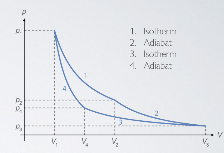
The fact that the efficiency of all reversible heat engines is the same means that we only need to calculate it once to get a universally valid expression for it. Moreover, we can do the calculation for a case that is designed to make that calculation easy. To that end, we’ll use the Carnot cycle (Fig. 14.2b), which consists of two isothermal and two adiabatic processes. As we’ve seen in the previous section, in an isothermal process the curve in the \(pV\) plane is given by \(p = N \kB T / V\), and because the change in internal energy depends only on the change in temperature, for an isothermal process the internal energy is constant (\(\mathrm{d}U = 0\), so \(\mathrm{d}Q = - \mathrm{d}W\)). For an adiabatic process, we found \(p V^\gamma = \mathrm{const}\), where \(\gamma = C_p/C_V\). Since \(\gamma > 1\), the line describing an adiabat in the \(pV\) plane is steeper than that describing an isotherm, and we can create a cycle.
Calculating the amount of work done and amounts of heat absorbed and extracted in a Carnot cycle is now a simple exercise. For the isothermal process from \((p_1, V_1)\) to \((p_2, V_2)\), we get (combining the ideal gas law, the expression for work in equation (13.2), and the isothermal property that \(\mathrm{d}Q = - \mathrm{d}W\))
Likewise, we find that the amount of heat dumped in the isothermal process from \((p_3, V_3)\) to \((p_4, V_4)\) is given by \(Q_\mathrm{c} = N \kB T_\mathrm{c} \log(V_3 / V_4)\). Since the two adiabatic processes occur (by construction) without absorbing or dumping any heat, we can write for the efficiency:
Now \(V_2\) and \(V_3\) (and \(V_4\) and \(V_1\)) are related by adiabatic processes, which obey \(p V^\gamma = \mathrm{const}\), or, again by application of the ideal gas law, \(T V^{\gamma - 1} = \mathrm{const}\), so we have \(T_\mathrm{h} V_2^{\gamma-1} = T_\mathrm{c} V_3^{\gamma-1}\) and \(T_\mathrm{h} V_1^{\gamma-1} = T_\mathrm{c} V_4^{\gamma-1}\). If we divide these two equations by each other, we find that \(V_2 / V_1 = V_3 / V_4\), which means that the two log terms in equation (14.16) are equal, and thus
Irreversible heat engines will necessarily have a lower efficiency (otherwise they could be used to break Carnot’s theorem). Practical heat engines, even when run at a close-to-reversible cycle, will also have a lower efficiency, as some of the work produced will necessarily dissipate due to friction.
14.3. Entropy#
We’ve arrived at last at the mysterious and often ill-understood concept of entropy. Let us start with two common misconceptions. The first is that entropy is a measure of ‘energy quality’, that is to say, that some energy would be more useful than others. The second is that entropy is a measure of disorder - a broken egg having higher entropy than an unbroken one. Neither of these is entirely wrong, but neither is entirely correct either. Indeed, if we are given a system with a (relatively) low entropy, we will be able to construct an engine to extract work from it. And also indeed, if you compare the molecules in a drop of ink that you’ve just put in a glass of water (the ‘more ordered’ state), to the later situation in which they’re dispersed throughout the water (the ‘less ordered’ state), the first has the lower entropy. However, counter-examples also exist. The best known one is probably the depletion interaction, in which you dissolve both relatively large colloids (spherical particles of, say, \(100\;\mu\mathrm{m}\) in diameter) and smaller polymers (which form blobs of say \(5\;\mu\mathrm{m}\)) in water - in that case, the colloids and polymers will spontaneously demix, and the demixed state has the highest entropy. Moreover, in this example the energy is constant, so the ‘quality of energy’ description doesn’t really apply either.
Then what is entropy? The simplest way to understand it is through a direct analogy with mechanics. In mechanics, the total energy consists of the sum of the kinetic and potential energy, and is conserved, like it is in thermodynamics. Potential energy is nothing but ‘the potential to do work’ (remember that the potential energy difference between A and B is simply minus the amount of work you need to do to transport something from A to B), and by the work-energy theorem, doing work results in a change of the kinetic energy. In thermodynamics, the entropy is analogous to the potential energy, with one important (historical) difference, namely its sign. While a higher potential energy means you can extract more work from the system, a lower entropy also means you can extract more work from the system. A mechanical system that is left alone will minimize its potential energy; a thermodynamic system that is left alone will maximize its entropy.
To find a way to calculate the entropy, we return to the Carnot cycle. We found that its efficiency is given by \(1-T_\mathrm{c}/T_\mathrm{h}\) (equation (14.17)). Comparing with the (14.13) of efficiency allows us to read off that \(Q_\mathrm{c}/Q_\mathrm{h} = T_\mathrm{c}/T_\mathrm{h}\), or, after rearranging
Remember that \(Q_\mathrm{h}\) is the heat that flows into the engine from the hot bath at \(T_\mathrm{h}\), whereas \(Q_\mathrm{c}\) is the heat that flows out of the engine to the cold bath at \(T_\mathrm{c}\). Equation (14.18) tells us that in a complete cycle, the difference between the ‘heat per temperature’ influx and outflux is zero. Therefore, in addition to the internal energy of the system, this ‘heat per temperature’ gives us a second quantity that is unchanged when we’ve gone through a full reversible cycle. This second quantity is the entropy.
You may object that, even though we’ve proven that the efficiency of any reversible engine must be the same, we used the specific setup of the Carnot engine to derive equation (14.17). For any other system (e.g., the isovolumetric/isobaric engine in Fig. 14.2a), heat does not flow in at a constant temperature, as the internal temperature of the engine changes under compression or expansion. You would of course be right, so we need a little care to make our expression for the entropy universally valid. The trick is to consider infinitesimal steps: let us add, reversibly, an infinitesimal amount of heat \(\delta Q\) from a reservoir at temperature \(T\). The added ‘heat per temperature’, or entropy, to the system is then given by
Adding heat to a system increases its entropy, removing heat (i.e., flipping the sign of \(\delta Q\)), removes it. For a complete Carnot cycle, we can integrate equation (14.19) to get
by equation (14.18).
We can always construct a Carnot cycle between any two points \((p_1, V_1)\) and \((p_2, V_2)\) in the \(p\), \(V\) state space of an engine. By equation (14.20), the entropy change if we go through the entire cycle is zero, so we can define an entropy difference between the two points as
where ‘1’ and ‘2’ refer to the points in the state space.
Equations (14.20) and (14.21) still wouldn’t be much use if the change in entropy would depend on the path taken. Fortunately, that is not the case: the entropy, like the energy, is a state function: it depends only on the thermodynamic variables[3]. You can easily see that this is true, as you can describe any cycle as the limit of a large number of Carnot cycles, and as equation (14.20) holds for each of those Carnot cycles, it also holds for their sum, i.e., the arbitrary cycle. Therefore, the change in entropy over any closed path is zero:
and the entropy difference between two points is well-defined.
As you have surely noticed, equations (14.22) and (14.21) are mathematically identical (except for the minus sign) to the equations for the work done by a conservative force along a closed path and the definition of the potential energy difference between any two points (see Section 3.3). When left to its own devices, a mechanical system, through friction and drag (non-conservative forces) will generally tend to find a local minimum of its potential energy. Likewise, thermal systems, by dissipating energy to their environment, will gradually tend to maximize their entropy. The equilibrium point (the equivalent to the minimum of the potential energy) is thus the state of maximum entropy.
The mathematical form of the above statement (i.e., that systems tend to maximize their entropy) is known as the Clausius theorem, which states that for any cycle, we have
where \(T_\mathrm{env}\) is the temperature of the environment (with which the system can exchange heat). When considering an infinitesimal step, we then get for the entropy of the system itself:
The proof of the Clausius theorem is not difficult (see Exercise 14.3): it essentially is a direct application of the second law of thermodynamics, as heat can only flow from a reservoir into the system if the reservoir is hotter than the system, and only from the system to a reservoir if the reservoir is colder than the system. These temperature differences can be a source of heat dissipation (resulting in an increase in overall entropy) without the production of work.
A direct consequence of the Clausius theorem is that the entropy in a closed system can never decrease. Considering the universe as a whole, we can also conclude that the entropy of the entire universe can never decrease (but it can, and does, increase over time). These observations are direct consequences of the second law of thermodynamics. Alternatively, one can prove the second law by taking the entropy observations as an axiom, an approach taken in many textbooks. The major downside of that approach is that the law by itself does not tell you what entropy is, resulting in the common confusion about its meaning.
14.4. Thermodynamic variables#
Systems in the thermodynamic limit (meaning that they consist of a very large number of constituent particles) can be described by a relatively small set of variables. We’ve encountered several of them above: the temperature, pressure, volume, and number of particles (or number of moles) in the system. We’ve also seen that these variables can be related to each other through an equation of state that describes the system at hand (with the ideal gas law as our main example). Finally, we’ve encountered two state functions, which are functions of these variables alone: the internal energy and the entropy. Here, we’ll dive into the relation between all these variables in some more detail, which will give us a universal relation between all of them.
When considering our thermodynamic variables, the first thing to note is that they come in two types. The first type doesn’t care about the volume of the system. If the air in a room is at a certain temperature and you put a wall in the middle of the room, the temperature in the two new subrooms will still be equal. The same goes for the pressure of the air. We call these variables intensive. The second type scales with the size of the system - double the size, and you double the variable. Examples are the volume and the number of particles. We call these variables extensive.
Unsurprisingly, the internal energy of a thermodynamic system is also an extensive variable. You can see this explicitly in the expression for the internal energy of an ideal gas (equation (14.4)), which scales with the number of moles of gas. Likewise, the heat flow \(Q\) and amount of work done \(W\) depend on the amount of gas. We already noted that the work is the product of a pair of conjugate variables (here the pressure and the volume); we now see that one of them is intensive, and the other extensive.
By its very definition, the entropy is also an extensive variable. As both energy and entropy are extensive, we may expect that changes in energy and entropy are related by an intensive variable, just like changes in volume and energy are related by the (intensive) pressure. To see how this works, consider a system with fixed volume \(V\) and number of particles \(N\). We then add an infinitesimal amount of heat \(\delta Q\) to this system. As the volume and number of particles are held fixed, there is no net work done, so by the first law, \(\mathrm{d}U = \delta Q\), and by combining this relation with equation (14.21), we get
Perhaps unsurprisingly, the intensive variable relating energy and entropy is the temperature. Temperature and entropy are thus another pair of conjugate variables. Equation (14.25), in combination with (13.2), allows us to re-write the first law in terms of entropy, volume, and number of particles:
Equation (14.26) is the form of the first law[4] that is most used. We introduced the third term, \(\mu \,\mathrm{d}N\), to allow for a change in the number of particles as well. \(N\) is a dimensionless extensive variable, so \(\mu\), known as the chemical potential, must be an intensive variable with the dimension of energy: it is simply the energy cost of adding one more particle at fixed volume and entropy.
Equation (14.26) tells us that we can write the internal energy \(U\) as a function of the entropy, volume, and number of particles: \(U = U(S, V, N)\). For each of these extensive variables, if we want to calculate the conjugate intensive variable, we take the derivative of \(U\) with the other variables kept fixed, so we have:
14.5. Free energy and order parameters#
14.5.1. Free energy#
We’ve seen in Section 14.2 and Section 14.3 that not all internal energy of a system is available to do work. In particular for a heat engine, some of the available energy in the hot reservoir will inevitably be used to raise the temperature of the cold reservoir, and thus the total entropy of the system consisting of the engine and whatever it is working on. This principle holds generally, as a direct consequence of the second law of thermodynamics. In many practical cases, knowing the internal energy of your system is therefore not very useful. Instead, you want to know how much energy is available to do work. This quantity is known as the (Helmholz) free energy[5], which is given by[6]
and its differential can easily be calculated to be
The Helmholz free energy is a function of the system’s temperature, volume, and number of particles. Like the internal energy, it is extensive, meaning that it scales with the system size. It is particularly useful for the study of solutions. There are, however, cases for which it is not the most useful choice, for example when studying gases. In that case, rather than controlling the volume, it may be easier to control the pressure of your system. Fortunately, there is also free energy that is a function of temperature, pressure, and number of particles, known as the Gibbs free energy, given by
Alternatively, you might have a system that, in addition to a reservoir of heat, has a reservoir of particles (a grand-canonical system) at a given chemical potential. In that case, the free energy would be a function of temperature, volume, and chemical potential, known as the grand canonical free energy
Finally, in chemistry you may encounter reactions which produce or absorb heat (so the temperature is not fixed), for which the free energy is a function of entropy, pressure, and number of particles: the enthalpy:
All the free energies defined above are extensive. Note that you cannot define a free energy that is a function of the temperature, pressure, and chemical potential: it would be a function of intensive variables alone, and thus no longer extensive, and therefore be the same for all system sizes.
14.5.2. Phase transitions and phase coexistence#
Large collections of particles can exhibit different levels of ordering dependent on thermodynamic parameters such as the temperature and pressure. These different levels of ordering are commonly referred to as phases. For a substance that consists of identical particles only (a single component system), these phases include solid, liquid and gas. We can draw a phase diagram for such a system as a function of temperature and pressure, indicating for which values of the parameters the system is in which state, as we did in Fig. 13.4. The boundaries between these values indicate phase transitions, at which the ordering of the system changes.

Fig. 14.4 Two coexisting phases that are separated by a boundary that allows for the transfer of heat, volume, and particles. In equilibrium, the entropy of the whole system will be maximized, resulting in a state in which the two phases have the same temperature, pressure, and chemical potential (see equation (14.36)).#
At a phase boundary, two phases coexist in a configuration which is in thermodynamic equilibrium. As we discussed in Section 13.1, thermodynamic equilibrium means that the system is in thermal, mechanical, and chemical equilibrium. For two coexisting phases, these conditions translate to the statements that their temperatures, pressures, and chemical potentials must be equal. We can prove this statement using the laws of thermodynamics. According to (the differential form of) the first law, equation (14.26), any change in energy of a system in equilibrium is due to a change in entropy, volume, or number of particles. From equation (14.26), we see that the energy itself is a function of entropy, volume, and particle number: \(U = U(S, V, N)\). We can invert this function to find an expression for the entropy, which then must be a function of the energy, volume, and particle number: \(S = S(U, V, N)\). The second law of thermodynamics now tells us that for any spontaneous process in a closed system, the entropy can only increase, \(\Delta S \geq 0\). Consequently, the entropy in a system in equilibrium is always maximized. Now suppose we have a closed system with two coexisting phases, separated by a movable, permeating and heat-conducting wall (Fig. 14.4). We label the energy, volume, and number of particles in the two subsystems with 1 and 2, and because the system is closed, \(U = U_1 + U_2\), \(V = V_1 + V_2\), and \(N = N_1 + N_2\) are conserved. For any process that transfers heat, volume, or particles from one subsystem to the other, we thus have \(\Delta U = \Delta U_1 = -\Delta U_2\), \(\Delta V = \Delta V_1 = -\Delta V_2\), and \(\Delta N = \Delta N_1 = -\Delta N_2\). For the change in entropy in the whole system as a result of this transfer, we can then write
Now because \(S\) attains a maximum at equilibrium, we must have \(\Delta S = 0\), which can only be satisfied if \(T_1 = T_2\), \(p_1 = p_2\), and \(\mu_1 = \mu_2\).
14.5.3. Order parameters and phase transitions#
A phase transition is usually related to the breaking of a symmetry of the system. Simple examples include the liquid-to-solid phase transition, in which translational symmetry is broken (liquids are homogeneous, while crystals only have a discrete symmetry), the demixing of two fluids (from a single to two coexisting homogeneous states) and the paramagnetic (isotropic) to ferromagnetic (ordered) transition, which leads to the creation of a magnet when cooling down certain metals or alloys (known as ferromagnets[7]). The breaking of such a symmetry is usually described by a change in a thermodynamic function known as the order parameter, with the defining property that they are different in each phase. Order parameters are usually (though not always) chosen such that they are zero in the more symmetric phase, and nonzero in the broken-symmetry phase. Unfortunately, there is no general procedure for selecting a ‘good’ (as in, easy to work with while physically accurate) order parameter; finding one that is appropriate to the system at hand is therefore a bit of an art. In some cases, the selection is easy though. For the onset of magnetization, we choose the net magnetization \(\bm{m}\), defined as the magnetic dipole moment per unit volume of the material. For the gas-to-liquid transition we use the density \(\rho\) (or the difference between the density and the density at coexistence, \(\rho - \rho_\mathrm{c}\)), and for the demixing transition the volume fraction \(\phi\) of one of the components as our order parameter.
As systems tend to spontaneously minimize their free energy (which free energy, like the order parameter, depends on the system), we can find the state of a system by minimizing the free energy as a function of the order parameter. Although we usually have no explicit expression for this function, close to a phase transition we can expand it in a Taylor series around the value at coexistence. This approach was pioneered by the Russian physicist Lev Landau, and is therefore known as Landau theory of phase transitions. We’ll illustrate the idea here with the simplest possible case, in which the free energy \(F\) is a symmetric function of an order parameter \(\phi\) close to the coexistence line. As constant terms are irrelevant in any energy, the first two nontrivial terms are then the square and fourth order terms in \(\phi\), and we can write
The function \(F_4(T)\) has to be strictly positive, as otherwise the energy would strictly decrease for large values of \(\phi\), and thus the system would automatically evolve to the limit that \(\phi\) diverges. The function \(F_2(T)\) can be negative or positive. In the latter case, we have a single minimum, but in the former case, we get two, with a local maximum in between at \(\phi = 0\); that is the case for which we find phase coexistence. In Fig. 14.5, some examples are plotted for free energies at various positions in the phase diagram close to the coexistence line of the liquid and gas phase.

Fig. 14.5 Phase diagram with sketches of the free energy close to and on the coexistence line, at the critical point, and ‘beyond’ the critical point (on the extrapolated coexistence line).#
If you move along the phase coexistence line in Fig. 14.5 (i.e., move from (c) to (e) to (f)), the local maximum gets less high, until it disappears at (f). There, the term \(F_2(T)\) in the Landau expansion (14.37) equals zero, and the corresponding \(F(\phi)\) curve is very flat in the center, as not only its first, but also its second and third derivatives vanish. Beyond this point, \(F_2(T)\) becomes positive, and only a single minimum remains (Fig. 14.5g). Point (f) is thus the critical point, where the difference between the liquid and gas phase disappears.
14.6. Relations between the intensive variables#
14.6.1. The Gibbs-Duhem relation#
Although we’ve split the concept of ‘thermodynamic equilibrium’ into three constitutive parts, in practice you can’t separate them fully. That is not due to lack of experimental skill, but due to a fundamental constraint in thermodynamics: a relation between the intensive variables of a system that fixes one of them as a function of the others. For example, in a single-component system, once you’ve set the temperature and pressure, the chemical potential is also set.
To derive the relation between the intensive variables, we’ll start from the Gibbs free energy, \(G = G(T, p, N)\), which is a function of two intensive variables, temperature and pressure, and a single extensive variable, the number of particles. Because any (free) energy is also extensive, we know that \(G\) must scale linearly with \(N\). We can therefore define a Gibbs free energy per particle, which is a function of \(T\) and \(p\) alone:
We can substitute \(G = N g\) in the expression for the differential \(\mathrm{d}G\) of \(G\), equation (14.31), to get an expression for the differential of \(g\):
Comparing equations (14.31) and (14.39), we can read off that
The Gibbs free energy per particle thus equals the chemical potential[8] (the energy you need to add a single particle). Substituting that equation into equation (14.40) gives us the Gibbs-Duhem relation between the intensive variables:
The Gibbs-Duhem relation can be extended to systems containing multiple components (the term on the left-hand side is then replaced by \(\sum_i N_i \,\mathrm{d}\mu_i\), with the sum running over all components). We can also formalize it one step further, and replace all extensive variables except the entropy with an abstract extensive variable \(X_i\) (sometimes called a ‘flux’), paired with an intensive variable \(f_i\) (called a ‘force’). In that case, the (internal) energy is a function of \(S\) and the \(X_j\)’s, the temperature is still \((\partial U/\partial S)_{X_i}\), and the forces are the other derivatives, \(f_i = (\partial U/\partial X_i)_{T,X_{j \neq i}}\). The Gibbs-Duhem relation then reads:
14.6.2. The Gibbs phase rule#
When you mix multiple components, additional phases appear, that are enriched in some of the components. Such phases may be solid, liquid or gaseous in nature, and like in the one-component case, multiple phases can coexist in equilibrium. Coexistence lines may also still end in critical points as a function of temperature, pressure, or another thermodynamic variable. Unlike the one-component case, more than two phases can coexist for a range of values of these variables. The maximum number of coexisting phases that can exist in a system is given by the Gibbs phase rule:
where \(C\) is the number of components, and \(F\) the number of degrees of freedom, i.e., the number of intensive variables (such as temperature and pressure) that can be varied simultaneously and arbitrarily without determining one another. For a one-component system, we can get at most three phases if we fix both temperature and pressure (i.e., put \(F=0\), at the unique triple point), while for a three-component system we could thus get up to five coexisting phases. The Gibbs phase rule follows from the fact that the intensive thermodynamic properties are not independent, as they are related by the Gibbs-Duhem relation (14.42). When the pressure and temperature are variable, the composition of a phase with \(C\) components is thus set by specifying \(C-1\) chemical potentials, as the last one follows from the Gibbs-Duhem relation. If there are \(P\) phases coexisting at a point, there are a total of \((C+1)P\) variables to be set (the \(C-1\) chemical potentials, the temperature, and the pressure in each phase) with \(C(P-1)+2(P-1)\) constraints, as the chemical potentials of all components, temperatures, and pressures must be equal across the phases. The number of degrees of freedom is given by the number of variables minus the number of constraints, which gives \(F = (C+1)P - C(P-1) - 2(P-1) = C - P + 2\), or equation (14.44).
14.7. Appendix: The internal energy of an ideal gas#
In this appendix we will show that the internal energy of an ideal gas is independent of its pressure and volume, and therefore a function of its temperature and number of particles only. This feature is a direct consequence of the equation of state of the ideal gas, also known as the ideal gas law (equation (13.17)): \(pV = N \kB T\). In our derivation, we make use of the differential form of the first law of thermodynamics (equation (14.26)), taking the number of particles to be constant, and writing \(\mathrm{d}U = T \,\mathrm{d}S - p \,\mathrm{d}V\). With the number of particles constant, the system in general is a function of two independent parameters, which we are free to choose. We choose the temperature (obviously) and the volume. Then \(U = U(T,V)\) and \(S = S(T,V)\), so
and
Since we have no expression for \(S\), we need to get an alternative for the derivative on the right of equation (14.46). We will do so using the Helmholz free energy, \(F = U - TS\), and the general mathematical properties of a total differential. Suppose we have a general function of two variables \(G(x,y)\), and its differential is given by \(\mathrm{d}G = X \mathrm{d}x + Y \mathrm{d}y\), then we have:
Applying this to the differentials of the various free energies and other thermodynamic functions leads to a range of very useful thermodynamic relations, known as the Maxwell relations. Here we will apply equation (14.47) to the differential of the Helmholz free energy, \(\mathrm{d}F = - S \,\mathrm{d}T - p \,\mathrm{d}V\), which gives
Substituting (14.48) in (14.46) and using the ideal gas law, we find
so the energy is indeed independent of the volume, and a function of the temperature alone. By integrating equation (14.49), we find that this is true for any equation of state of the form
where \(f(V)\) is any function of \(V\), as long as it is independent of \(T\). Equation (14.49) still holds and the internal energy is a function of the temperature alone. Specifically, this result also holds for the van der Waals gas, which is an equation of state for a fluid consisting of particles that are not finite and do exert pairwise attractive forces (such as the van der Waals force) on each other. The van der Waals equation of state is given by
where \(a\) is a measure of the attraction between the particles, and \(b\) the volume excluded by a particle.
14.8. Problems#
Exercise 14.1 (A simple heat engine)
Possibly the simplest heat engine is the ‘square cycle’ in Fig. 14.2a.
Find the efficiency of this heat engine.
The efficiency you found at (a) is lower than that of a Carnot cycle operating between the same two temperature extremes. Why does this engine not break Carnot’s theorem?
Exercise 14.2 (Stirling engine)
Building a Carnot engine, although theoretically possible, is practically challenging. A much simpler design that yet works well is the Stirling engine, see figure. The corresponding cycle consists of four steps: (1) Isothermal expansion, (2) Isovolumetric cooling, (3) Isothermal compression and (4) Isovolumetric heating.
Draw the Stirling cycle in a (\(p, V\)) diagram.
Calculate the values of the pressure and volume at each of the vertices of the cycle if the cold reservoir is at \(T_\mathrm{c}\), the hot reservoir at \(T_\mathrm{h}\), and the initial pressure and volume are \(p_1\) and \(V_1\), respectively.
Calculate the amount of work that can be extracted in a Stirling cycle.
Show that the theoretical efficiency of the Stirling cycle is identical to that of the Carnot cycle (as it should be based on Carnot’s theorem).
Exercise 14.3 (The Clausius theorem for cyclic processes)
The Clausius theorem states that in any cyclic process (both reversible and irreversible), we have (equation (14.23)):
where \(T_\mathrm{surr}\) is the temperature of the environment. Equivalently, for each infinitesimal step, the entropy change of the system itself needs to be larger or equal to that of the environment (equation (14.24)):
To prove the theorem, we first consider a step in which the system absorbs heat from the environment without any work being done. Argue that for that to be possible, the temperature of the environment, \(T_\mathrm{surr}\), must be higher than that of the system at this point, \(T_1\), and from that show that minus the decrease in the entropy of the environment, \(-\mathrm{d}S_\mathrm{surr}\) must be less than or equal to the increase in entropy of the system, \(\mathrm{d}S_\mathrm{sys}\).
Likewise, consider a step in which the system (now at a higher temperature \(T_2\)) expels heat to the environment, and show that for such a step, the increase in the entropy of the environment must be greater than or equal to minus the decrease in the entropy of the system.
From your results at (a) and (b), show that
\[- \oint \mathrm{d}S_\mathrm{surr} \leq \oint \mathrm{d}S_\mathrm{sys}.\]By relating the change in entropy of the environment to the heat flow, show that if the system itself goes through a reversible cyclic process, the heat flow from the environment to the system must satisfy the Clausius theorem, equation (14.23).
Finally, invert the statement in (d) to show that any system left alone and free to exchange heat with its environment will always tend to maximize its entropy.