
4. Momentum#
4.1. Center of mass#
4.1.1. Center of mass of a collection of particles#
So far we’ve only considered two cases - single particles on which a force is acting (like a mass on a spring), and pairs of particles exerting a force on each other (like gravity). What happens if more particles enter the game? Well, then we have to calculate the total force, by vector addition, and total energy, by regular addition. Let’s label the particles with a number \(\alpha\), then the total force is given by:
where we’ve defined the total mass \(M = \sum_\alpha m_\alpha\) and the center of mass
4.1.2. Center of mass of an object#
Equation (4.2) gives the center of mass of a discrete set of particles. Of course, in the end, every object is built out of a discrete set of particles, its molecules, but summing them all is going to be a lot of work. Let’s try to do better. Consider a small sub-unit of the object of volume \(\mathrm{d}V\) (much smaller than the object, but much bigger than a molecule). Then the mass of that sub-unit is \(\mathrm{d}m = \rho \mathrm{d}V\), where \(\rho\) is the density (mass per unit volume) of the object. Summation over all these masses gives us the center of mass of the object, by equation (4.2). Now taking the limit that the volume of the sub-units goes to zero, this becomes an infinite sum over infinitesimal volumes - an integral. So for the center of mass of a continuous object we find:
Note that in principle we do not even need to assume that the density \(\rho\) is constant - if it depends on the position in space, we can also absorb that in the discussion above, and end up with the same equation, but now with \(\rho(\bm{r})\). That will make the integral a lot harder to evaluate, but not necessarily impossible. Also note that the total mass \(M\) of the object is simply given by \(\rho \cdot V\), where \(V\) is the total volume, if the density is constant, and by \(\int_V \rho(\bm{r}) \mathrm{d}V\) otherwise. Therefore, if the density is constant, it drops out of equation (4.3), and we can rewrite it as
Unfortunately, many textbooks introduce the confusing concept of a infinitesimal mass element \(\mathrm{d}m\), instead of a volume element \(\mathrm{d}V\) with mass \(\rho \mathrm{d}V\). This strange habit often throws students off, and the concept is wholly unnecessary, so we won’t adapt it here.
Equation (4.3) holds for any continuous object, but it might be confusing if you consider a linear or planar object - as you may wonder how the density \(\rho\) and volume element \(\mathrm{d}V\) are defined in one and two dimensions. There are two ways out. One is to say that all physical objects are three-dimensional - even a very thin stick has a cross section. If you say that cross section has area \(A\) (which is constant along the stick, or the thin stick approximation would be invalid), and the coordinate along the stick is \(x\), the volume element simply becomes \(\mathrm{d}V = A \mathrm{d}x\), and the integral in equation (4.3) reduces to a one-dimensional integral. You can approach two-dimensional objects in the same way, by giving them a small thickness \(\Delta z\) and writing the volume element as \(\mathrm{d}V = \Delta z \mathrm{d}A\). Alternatively, you can define one- and two-dimensional analogs of the density: the mass per unit length \(\lambda\) and mass per unit area \(\sigma\), respectively. With those, the one- and two-dimensional equivalents of equation (4.3) are given by
where \(M\) is still the total mass of the object.

Example 4.1 (center of mass of a solid hemisphere)

Fig. 4.1 Coordinate system for the calculation of the center of mass for a solid hemisphere.#
By symmetry, the center of mass of a solid sphere must lie at its center. The center of mass of a hemisphere cannot be guessed so easily, so we must calculate it. Of course, it must still lie on the axis of symmetry, but to calculate where on that axis, we’ll use equation (4.4). To carry out the integral, we’ll make use of the symmetry the system still has, and chop our hemisphere up into thin slices of equal thickness \(\mathrm{d}z\), see Fig. 4.1. The volume of such a slice will then depend on its position \(z\), and be given by \(\mathrm{d}V = \pi r(z)^2 \mathrm{d}z\), where \(r(z)\) is the radius at height \(z\). Putting the origin at the bottom of the hemisphere, we easily obtain \(r(z) = \sqrt{R^2 - z^2}\), where \(R\) is the radius of the hemisphere. The position vector \(\bm{r}\) in equation (4.4) simply becomes \((0, 0, z)\), so we get:
The center of mass of the solid hemisphere thus lies at \(\bm{r}_\mathrm{cm} = (0, 0, 3R/8)\).
4.2. Conservation of momentum#
In equation (4.1), what is the total force acting on all the particles? Well, that’s the sum of all the forces the particles exert on each other, plus all external forces: \(\bm{F}_\mathrm{total} = \sum_i \bm{F}_{\mathrm{int},i} + \sum_i \bm{F}_{\mathrm{ext}, i}\). Now Newton’s third law of motion tells us that the internal forces come in opposite pairs, so when we sum them, they all cancel, and the total net force acting on the particles is equal to the sum of the external forces acting on the particles. Therefore, by equation (4.1), the center of mass of a system of particles obeys Newton’s second law of motion.
What about the momentum of the center of mass? Like the force, the total momentum of the system of the system is given by the vector sum of the individual particle momenta:
so the total momentum of the system equals that of the center of mass. Moreover, as long as the mass of the system is conserved, we can rewrite equation (4.1) as
Not only does the center of mass of a system of particles obey Newton’s second law of motion, its total momentum does too. Moreover, unlike in the single-particle case, equation (4.7) has an important consequence for the case that there is no external force acting on the system. For one particle, that would simply mean that the momentum does not change - Newton’s first law of motion. But for multiple particles, equation (4.7) tells us that no external forces means that the total momentum does not change. We have therefore arrived at our second conservation law:
Theorem 4.1 (Law of conservation of momentum)
When no external forces act on a system of particles, the total momentum of the system is conserved.
We derived the law of conservation of momentum by applying both Newton’s second and third laws of motion, so like conservation of energy, it is not an independent result, but follows from our axioms. Note that the law allows for the momenta of the individual particles in the system to change, as long as their total stays the same - this is what happens when you play billiards, and why the number of balls bouncing in a Newton’s cradle is fixed.
4.3. Reference frames#
4.3.1. Center of mass frame#
The center of mass need not be fixed in space, so it can have a nonzero velocity, which of course is simply given by \(\bm{v}_\mathrm{cm} = \dot{\bm{r}}_\mathrm{cm}\). For each of the particles in a multi-particle system, we can decompose its velocity by writing it as the sum of the center of mass velocity and a velocity relative to the center of mass:
In many applications, the information is in the velocity component relative to the center of mass. After all, conservation of momentum implies that for a system with no external forces acting on it, the center of mass velocity cannot change, even if all the individual momenta do change (as happens in collisions). Therefore, it is often convenient to analyze your system in a frame that moves with the center of mass, known (unsurprisingly), as the center of mass frame. In this frame, the center of mass velocity is identically zero, and again because of conservation of momentum, all other velocities in this frame must sum to zero. The ‘real-world’ frame with nonzero center of mass velocity is referred to as the lab frame.
4.3.2. Galilean transformations and inertial frames#
As equation (4.8) shows, if you know a particle’s velocity in the center of mass frame, you can easily calculate the velocity in the lab frame by adding the velocity of the center of mass. Going the other way, to calculate the velocity in the center of mass frame, you subtract \(\bm{v}_\mathrm{cm}\) from the velocity in the lab frame. Moreover, if the center of mass moves at constant velocity, we can also easily relate positions in both frames. If we denote coordinates in the lab frame by \(\bm{r}\) and those in the center of mass frame by \(\bm{r}'\), we readily obtain:
Equation (4.9) is an example of a Galilean transformation between frames of reference (here the lab frame and the center of mass frame). It actually holds for any pair of reference frames that move with constant velocity with respect to each other. Such frames of reference are known as inertial frames if Newton’s first law of motion holds in them; by Newton’s second law, if one of the frames is an inertial frame, then the one obtained from it by a Galilean transformation (i.e., one moving at constant velocity with respect to the first frame) is also an inertial frame. The reason for this is that a constant velocity plays no role in Newton’s second law, as it relates the derivative of the velocity (i.e., the acceleration) to a force. Consequently, not only is Newton’s first law of motion valid in both inertial frames - all laws of physics are the same in two such frames. This fact is known as the principle of relativity. It does not apply to, for example, frames that rotate with respect to each other, as we’ll see in Section 7. Moreover, although the principle of relativity is universally valid (it is in fact one of the two basic assumptions behind Einstein’s theory of relativity), the Galilean transformations are not. They break down at velocities that approach the speed of light, as discussed in part II of Mechanics and Relativity.
4.3.3. Kinetic energy of a collection of particles#
We’ve established above that both the total momentum and energy are conserved in closed systems, but the components can of course change. Momentum can be transferred from one particle to another, and so can (kinetic) energy; moreover kinetic energy can be generated from potential energy. Unfortunately, unlike momentum, the kinetic energy of a collection of particles does not equal that of the center of mass - this is because kinetic energy depends quadratically rather than linearly on the velocity. The total kinetic energy does of course equal the sum of the individual particles’ kinetic energies. Moreover, here too the decomposition (4.8) is useful:
Because the center of mass velocity is the same for all particles, it can be taken out of the sum in the second line. Therefore, the first term equals \(\frac12 M v_\mathrm{cm}^2 = K_\mathrm{cm}\), and in the second term we end up with the sum over all velocities relative to the center of mass - which is zero. We find that the total kinetic energy of a collection of particles equals the kinetic energy of the center of mass plus the total internal kinetic energy - which can change in both collisions and when potential energy gets converted into kinetic energy (or vice versa).
4.4. Rocket science *#
Although designing a rocket that will follow a desired trajectory (say to Ceres, Pluto, or Planet Nine) with great accuracy is an enormous engineering challenge, the basic principle behind rocket propulsion is remarkably simple. It essentially boils down to conservation of momentum, or, equivalently, the observation that the velocity of center of mass of a system does not change if no external forces are acting on the system. To understand how a rocket works, imagine[1] the following experiment: you sit on a initially stationary cart with a large amount of small balls. You then pick up the balls one by one, and throw them all in the same direction with the same (preferably high) speed (relative to yourself and thus the cart). What will happen is that you, the cart, and the remaining balls slowly pick up speed, in the opposite direction from the one you’re throwing the balls in. This is exactly what a rocket engine does: it thrusts out small particles (molecules, actually) at high velocities, gaining a small velocity itself in the opposite direction. Note that this is completely different from most other engines, which drive the rotation of wheels (that depend on friction to work) or propellers (that depend on drag to work).
4.4.1. Rocket equation#
To understand what happens in our thought experiment, let’s first consider the first ball you throw. Let’s call the mass of yourself plus the cart \(M\), the total mass of the balls \(m\), and the (small) mass of a single ball \(\mathrm{d}m\). If you trow the ball with a speed \(u\) (with respect to yourself), we can calculate your resulting speed in two ways:
The center of mass must remain stationary. Let’s put \(x_\mathrm{cm} = 0\). Before the throw, we then have \(x_\mathrm{ball} \mathrm{d}m + x_\mathrm{car} (M+m) = 0\), whereas after the throw we have \(-u t \mathrm{d}m + v_\mathrm{car} t (M+m) = 0\), or \(v_\mathrm{car} = - u \mathrm{d}m / (M+m)\).
The total momentum must be conserved. Before the throw, the total momentum is zero, as nothing is moving. After the throw, we get: \(p_\mathrm{ball} + p_\mathrm{car} = -u \mathrm{d}m + v_\mathrm{car} (M+m)\). Equating this to zero again gives \(v_\mathrm{car} = - u \mathrm{d}m / (M+m)\).
Now for the second, third, etc. ball, the situation gets more complicated, as the car (including the ball that is about to be thrown) is already moving. Naturally, the center of mass of the car plus all the balls remains fixed, as does the total momentum of the car plus all the balls. However, to calculate how much extra speed the car picks up from the \(n\)th ball, it is easier to not consider the balls already thrown. Instead, we consider a car (including the remaining balls) that is already moving at speed \(v\), and thus has total momentum \((M+m)v\). Throwing the next ball will reduce the mass of the car plus balls by \(\mathrm{d}m\), and increase its velocity by \(\mathrm{d}v\). Conservation of momentum then gives:
where we dropped the second-order term \(\mathrm{d}m \mathrm{d}v\). Equation (4.12) can be rewritten to
Note that here both \(u\) (the speed of each thrown ball) and \(M\) (the mass of yourself plus the car, or the shell of a rocket) are constants, whereas \(m\) changes, ending up at zero when you’ve thrown all your balls. To find the velocity of our car, we can integrate equation (4.13), but there is an important, and rather subtle, point to consider. The left-hand side of equation (4.13) applies to the car, but the right-hand side to the thrown ball, with a (positive) mass \(\mathrm{d}m\). The mass \(m\) of the balls remaining in the car, however, has decreased by \(\mathrm{d}m\), so if we wish to know the final velocity of the car, we need to include a minus sign on the right-hand side of equation (4.13). Dividing through by \(M+m\) and integrating, we then obtain:
where \(v_\mathrm{f}\) is the final velocity of the car, and \(m_0\) the initial total mass of all the balls. Equation (4.14) is known as the Tsiolkovsky rocket equation[2].
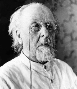
Konstantin Eduardovich Tsiolkovsky (1857-1935)
Konstantin Eduardovich Tsiolkovsky (1857-1935) was a Russian rocket scientist, who is considered to be one of the pioneers of cosmonautics. Self-taught, Tsiolkovsky became interested in spaceflight both through ‘cosmic’ philosopher Nikolai Fyodorov and science-fiction author Jules Verne and considered the construction of a space elevator inspired by the then newly built Eiffel tower in Paris. Working as a teacher, he spent much of his free time on research, developing the rocket equation named after him (equation (4.14)) as well as developing designs for rockets, including multi-stage ones. Tsiolkovsky also worked on designing airplanes and airships (dirigibles), but did not get support from the authorities to develop these further. He kept working on rockets though, while also continuing as a mathematics teacher. Only late in life did he receive recognition for his work at home (then the Soviet Union), but his ideas would go on to influence other rocket pioneers in both the Soviet and American space programs.
4.4.2. Multi-stage rockets#
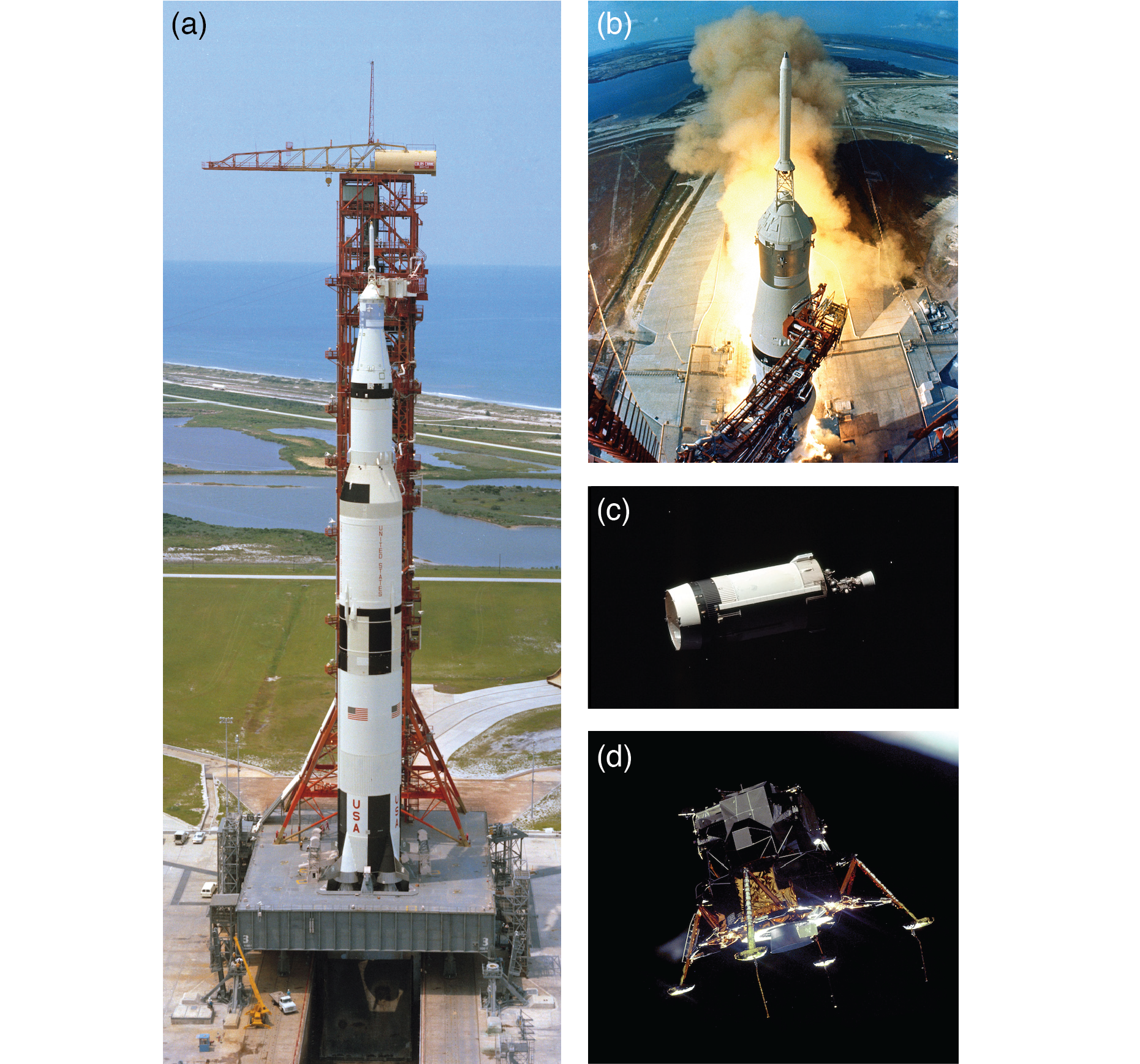
Fig. 4.3 Rockets and related spacecraft that took people to the moon in the late 1960’s and early 1970’s [4]. (a) Aerial view of a Saturn V rocket on its launchpad. This rocket carries the Apollo 15, the fourth mission to make it to the moon. The three rocket stages are separated by rings around the engine of the next stage. The total height of the rocket at launch was 110.6 m; it had a total mass of 2.97 million kg, and could take a payload of 140000 kg to low-Earth orbit or a payload of 48600 kg to the moon. (b) View from the launch tower of the Saturn V carrying Apollo 11 (the famous first mission to the moon in 1969) at ignition. The little rocket on top was to be used for an emergency escape of the manned module immediately below if anything went wrong at launch. The manned ‘command module’ is the little conical structure; the cylindrical structure directly below it contained its engine, and the conical part below that contained the lunar lander (figure d). (c) Jettisoned third stage of the Saturn V rocket that carried the Apollo 17 mission (the sixth and last(!) to make it to the moon in 1972). The empty space at the front contained the lunar lander module at launch. (d) Lunar lander of the 1969 Apollo 11 mission, photographed from the command module after separation. This module contained two rockets: one to slow the descent to the moon on the lower part, and one to return to moon orbit with just the upper part. The lower part of the lander remains on the moon and was photographed there in 2012 by the Lunar Reconnaisance Orbiter, an unmanned spacecraft in Moon orbit.#
Because of the logarithmic factor in the Tsiolkovsky rocket equation, rockets need a lot of fuel compared to the mass of the object they intend to deliver (the payload - say a probe, or a capsule with astronauts). Even so, the effectiveness of rockets is limited. A fuel to payload ratio of 9:1 (already quite high) and an initial speed of zero gives a final speed \(v_\mathrm{f} = u \log(10) \simeq 2.3 u\), and increasing the ratio to 99:1 only doubles this result: \(v_\mathrm{f} = u \log(100) \simeq 4.6 u\). To get around these limitations and give rockets (or rather their payloads) the speed necessary to leave Earth, or even the solar system, rockets are built with multiple stages - essentially a number of rockets stacked one upon the next. If these stages all have the same fuel to payload ratio and exhaust velocity, the final velocity of the payload simply is that of a single stage times the number of stages \(n\): \(v_\mathrm{f} = n u \log(1+m_0/M)\). To see this, consider that the remaining stages are the payload of the current stage. Having multiple stages thus allows rockets to pick up speed more efficiently, essentially by shedding a part of the ‘payload’ (casing of an empty stage). For example, the Saturn V rocket that was used to send the Apollo astronauts to the moon had three stages, plus a small rocket engine on the capsule itself (used to break moon orbit and send the astronauts back to Earth), see Fig. 4.3.
4.4.3. Impulse#
When you’re crashing into something, there are two factors that determine how much your momentum changes: the amount of force acting on you, and the time the force is acting. The product is known as the impulse, which by Newton’s second law equals the change in momentum:
The specific impulse, defined as \(I_\mathrm{sp} = J/m_\mathrm{propellant}\), or the impulse per unit mass of fuel, is a measure of the efficiency of jet engines and rockets.
4.5. Collisions#
Collisions occur when two (or more) particles hit each other. During a collision, those particles exert forces on each other, but in general, there are no external forces acting on the system consisting of the colliding particles. Consequently, the total momentum of all particles involved in the collision is conserved. Typically, we know the initial velocities and the masses of the particles, and want to calculate their final velocities - though of course you could also do it the other way around.
Although the total momentum of colliding particles is conserved, the total (kinetic) energy of all particles typically is not, as irreversible processes (such as plastic deformations of the particles) occur that are associated with nonconservative forces. In the special case that kinetic energy is conserved in a collision, we call the collision (totally) elastic. All other collisions are called inelastic, with the extreme case of a totally inelastic collision, in which the colliding objects stick together.
4.6. Totally inelastic collisions#
For the case of two particles colliding totally inelastically, conservation of momentum gives:
If the masses and initial velocities of the particles are known, calculating the final velocity of the composite particle is thus straightforward.

Example 4.2 (bike crash)
You’re late for class and it’s raining to boot, so you cycle as fast as you possibly can, without paying attention in which direction you’re going. A classmate, similarly late, comes towards you from a side street that makes an angle \(\phi\) with yours. When your streets cross, you crash into each other, moving together in a big clutch of people and bikes, see Fig. 4.4. Suppose you’re about equally heavy, but you’re the faster biker, with initially twice the speed of your classmate. Find the velocity (i.e., magnitude and direction) you and your classmate have immediately after the collision.

Fig. 4.4 Two colliding cyclists.#
Solution Let’s call your (and your classmate’s) mass \(m\), your initial speed \(2v\) (so your classmate’s speed is \(v\)), and your combined final speed \(v_\mathrm{f}\), with an angle \(\theta\) with your initial direction. After the collision you move as one object, so the collision is completely inelastic. During the collision we have conservation of momentum in both the \(x\) and \(y\) directions, which gives:
We need to solve for both \(v_\mathrm{f}\) and \(\theta\). To eliminate \(\theta\), we square both (4.17) and (4.18) and add them, which gives
or \(v_\mathrm{f} = v \sqrt{5-4\cos\phi}\). To get \(\theta\), we divide (4.17) by (4.18), which gives
We can easily check that these answers make sense when \(\phi=0\), which gives \(v_\mathrm{f} = v\) and \(\theta = 0\), as it should.
4.7. Totally elastic collisions#
For a totally elastic collision, we can invoke both conservation of momentum and (by definition of a totally elastic collision) of kinetic energy. We also have an additional variable, as compared to the totally inelastic case, because in this case the objects do not stick together and thus get different end speeds. The two equations governing a totally elastic collision are:
for momentum conservation, and
for kinetic energy conservation. Note that the squares in equation (4.20) represent a dot product of the vector with itself, a property which will be important when we study collisions in multiple dimensions.
4.7.1. Totally elastic collision in one dimension#
When the collision occurs in one dimension, we can combine equations (4.19) and (4.20) to calculate the final velocities as functions of the initial ones. We first rewrite the two equations so that everything associated with particle 1 is on the left, and the terms for particle 2 are on the right:
and
We can expand the terms in parentheses in equation (4.22), which gives:
Dividing equation (4.23) by equation (4.21), we get a relation between the velocities alone:
From equation (4.24) we can isolate \(v_{2,\mathrm{f}}\) and substitute back in (4.21) to find \(v_{1,\mathrm{f}}\) in terms of the initial velocities:
Naturally, we could just as well have calculated \(v_{2,\mathrm{f}}\), the equation for which is just (4.25) with the 1’s and 2’s swapped:
We note that in the limit case that \(m_2 \gg m_1\), \(v_2\) is hardly affected, and \(v_{1,\mathrm{f}} \simeq -v_{1,\mathrm{i}} + 2 v_{2,\mathrm{f}}\).
4.7.2. Elastic collisions in the COM frame#
Equations (4.25) and (4.26) give the final velocities of two particles after a totally elastic collision. We did the calculation in the lab frame, i.e., from the point of view of a stationary observer. We could of course just as well have done the calculation in the center-of-mass (COM) frame of Section 4.3. Within that frame, as we’ll see below, the relation between the initial and final velocities in an elastic collision is much simpler than in the lab frame.
We will use equation (4.8) to calculate velocities in the COM frame. For notational simplicity, we’ll work in one dimension, and use an overbar to indicate velocities in the COM frame, so we get
for each particle \(i\). The velocity of the center of mass is simply the time derivative of its position. For two particles, it is given by
The velocities of the two particles in the COM frame is then
where \(v_\mathrm{rel} = v_1 - v_2 = \bar{v}_1 - \bar{v}_2\) is the relative velocity of the two particles[5]. Note that it does not matter whether we calculate the relative velocity in the lab or COM frame. Equations (4.28) and (4.29) have a nice symmetry in their velocity components, but not in their mass components. The symmetry is more complete if instead of velocities, we consider momenta in the COM frame, where \(\bar{p} = m \bar{v}\):
where we introduced a new variable \(\mu\), the reduced mass
Clearly the total momentum in the center of mass frame is zero[6] (as it should be), both before and after a collision, and is thus conserved. To find out what happens with the relative velocity in an elastic collision, we invoke conservation of kinetic energy, which we calculate using \(K = \frac12 m v^2 = p^2 / 2m\):
We find that either \(\bar{v}_{\mathrm{rel},\mathrm{f}} = \bar{v}_{\mathrm{rel},\mathrm{i}}\), in which case there would be no collision (as nothing changes), or \(\bar{v}_{\mathrm{rel},\mathrm{f}} = - \bar{v}_{\mathrm{rel},\mathrm{i}}\), which means that in an elastic collision in the COM frame, the velocities (and momenta) of the colliding particles reverse. We get:
We can of course transform these expressions back to the lab frame by adding the center of mass velocity (4.27), which gives equations (4.25) and (4.26), the same as our calculation in the lab frame.
4.7.3. Totally elastic collision in multiple dimensions *#
If you write out equations (4.19) and (4.20) in two dimensions, you will end up with an underdetermined system: there are three equations, but four unknowns (the four components of \(\bm{v}_{1,\mathrm{f}}\) and \(\bm{v}_{2,\mathrm{f}}\)). In three dimensions, we add one more equation, but two more unknowns, so the situation gets even worse. We therefore are in need of an extra relation between the colliding particles. Fortunately, for the case that the particles are frictionless, the condition is easy: if there are no frictional forces, the only forces the particles can exert on each other are perpendicular to their contact surface. We will consider this friction-free case here; if there is friction, the particles will exert a torque on each other, resulting in a transfer of angular momentum, as we will study in Section 5.

Fig. 4.5 Two spheres colliding totally elastically. The total momentum is the same before (a) and after (c) the collision. During the collision, the spheres exert forces only along the line connecting their centers, perpendicular to their contact surface (dotted black line). The line connecting the centers lies along the normal \(\bm{\hat{n}}\), the plane is spanned by one (in 2D) or two (in 3D) tangent vectors \(\bm{\hat{t}}\). There is no change of velocities along any of the tangent directions; along the normal direction, the collision is equivalent to a fully elastic collision in one dimension.#
For general objects, finding the contact surface can be quite a challenge. For spheres however, it is easy: the contact surface is perpendicular to the line connecting the centers of the two colliding spheres. In two dimensions, the surface is a line, whereas in three dimensions, it is a plane. In both cases, the only forces acting between the spheres are along the line between their centers, which we will call the normal direction (because it is normal to the surface). The key point to finding the velocities of the spheres after the collision is now the observation that in any direction that there is no force, by Newton’s first law, there can be no change in the velocity. Therefore, we should decompose the velocities of the spheres in directions normal and tangential to the contact surface, see Fig. 4.5. The components of the velocity in any tangential direction (one in two dimensions, two in three dimensions) will simply be the same before and after the collision. Only the velocity in the normal direction changes, and in that direction, the particles are executing a one-dimensional elastic collision (which we solved already).
Finding the direction of the normal is easy for two spheres, as it is simply that of the line connecting their centers. A proper normal vector is normalized, so we have
where \(\bm{r}_1\) and \(\bm{r}_2\) are the positions of the two spheres. In two dimensions, we have
Finding the tangent vector is easy in two dimensions, as the only condition is that it should be perpendicular to the normal; we get
In three dimensions, getting two vectors that span the tangent plane is a bit more work; one way is to pick a vector that has \(0\) as the \(z\) component, and construct the \(x\) and \(y\) components like the 2D case; the second tangent vector can then be found as the cross product between the first tangent vector and the normal.
Once we have the normal and tangent vectors, we can decompose our velocities through projection[7]:
As explained above, because there are no tangential forces, there is no change of the velocity in the tangent direction, and we can immediately write down
Equation (4.38) is essentially the extra equation we need to solve the system of equations given by conservation of momentum (4.19) and of kinetic energy (4.20). Substituting it in these equations, we find that the conservation equations reduce to the one-dimensional ones for the components in the normal direction. We already found the solutions to these in Section 4.7.1, they are given by equations (4.25) and (4.26):
We now use equation (4.37) to combine the final normal and tangential components of the velocity back into a vector. The resulting expression can be written directly in terms of the initial velocities and the positions of the two spheres at the collision:
4.8. Partially elastic collisions#
In many real-life collisions, some of the kinetic energy is lost due to internal friction of the colliding objects. For example, a ball bouncing on the floor will deform during the collision, causing parts of the ball to move with respect to each other. The friction between those parts will lead to some work being done, resulting in the conversion of mechanical energy to heat, and causing the ball to bounce to a lower height than before. The amount of ‘inelasticity’ is measured by the coefficient of restitution, which is defined as the ratio of the relative velocities between the colliding objects after and before the collision:
For a completely elastic collision, we have \(C_\mathrm{R}=1\), and for a completely inelastic one, we have \(C_\mathrm{R}=0\) (though we can have \(C_\mathrm{R}=0\) also for a collision where the objects do not stick together). For a one-dimensional collision, we can combine equation (4.41) with conservation of momentum (4.19) to find the final velocities, which generalize equations (4.25) and (4.26) for the fully elastic collision:
As long as there are no frictional forces between the colliding particles, the extension to multiple dimensions goes in exactly the same manner as for totally elastic collisions.
4.9. Problems#
Exercise 4.1 (Celestial centers of mass)
We say that the Moon orbits the Earth, because the Earth’s gravity pulls on the Moon, causing it to orbit. However, by Newton’s third law, the Moon exerts a force back on the Earth. Therefore, the Earth should move in response to the Moon. Thus a more accurate statement would be that the Moon and the Earth both orbit the center of mass of the Earth-Moon system. Useful values: \(M_\mathrm{E} = 5.97 \cdot 10^{24}\;\mathrm{kg}\), \(R_\mathrm{E} = 6.37 \cdot 10^6\;\mathrm{m}\), \(R_\mathrm{E, orbit} = 1.50 \cdot 10^{11}\;\mathrm{m}\), \(M_\mathrm{M} = 7.35 \cdot 10^{22}\;\mathrm{kg}\), \(R_\mathrm{M} = 1.74 \cdot 10^6\;\mathrm{m}\), \(R_\mathrm{M, orbit} = 3.84 \cdot 10^{8}\;\mathrm{m}\), \(M_\mathrm{S} = 1.99 \cdot 10^{30}\;\mathrm{kg}\), \(R_\mathrm{S} = 6.96 \cdot 10^8\;\mathrm{m}\).
Find the center of mass of the Earth-Moon system (in an appropriately chosen, and clearly defined, coordinate system). Does this center of mass lie inside the Earth?
Find the location of the center of mass of the Earth-Moon-Sun system during a full Moon.
Find the location of the center of mass of the Earth-Moon-Sun system when the Moon is in its first quarter.
Exercise 4.2 (Exploding shell)
A shell is shot with an initial velocity of \(20\;\mathrm{m}/\mathrm{s}\), at an angle of \(60^\circ\) with the horizontal. At the top of the trajectory, the shell explodes into two fragments of equal mass. One fragment, whose speed immediately after the explosion is zero, drops to the ground vertically. How far from the gun does the other fragment land (assuming no air drag and level terrain)?
Exercise 4.3 (Two cannonballs)
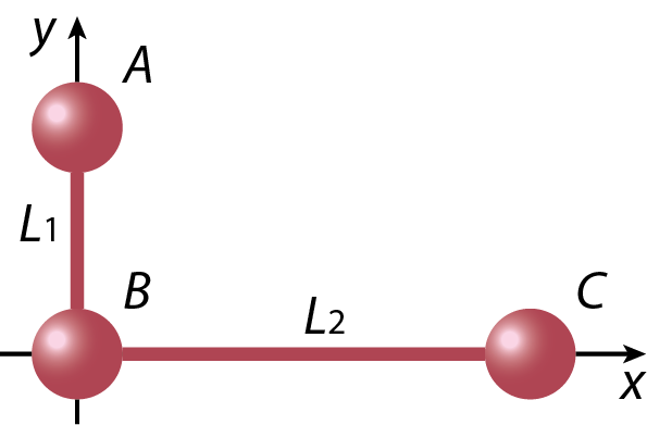
Two cannonballs with masses \(m_1\) and \(m_2\) are simultaneously fired from two cannons situated a distance \(L\) apart.
Find the equations of motion for the horizontal and vertical components of the vector describing the center of mass of the cannonballs.
Show that the motion of the center of mass is a parabola through space.
Exercise 4.4 (Center of mass of some solid objects)
Center of mass of some solid objects

Find the center of mass of an isosceles triangle with a base width \(w\) and height \(h\) (see figure a).
Find the center of mass of a pentagon with five equal sides of length \(a\), but with one triangle missing (see figure b). Hint: use your result from (a).
Find the position of the center of mass of a semicylinder (half of a solid cylinder, i.e., a solid cylinder sliced in two along a plane containing its symmetry axis). Hint: first calculate the center of mass of half a solid disk.
Exercise 4.5 (A dog walking in a boat)
A dog (black dot in the sketch below) of mass \(m\) stands at the end of a boat of mass \(M\) and length \(L\) at an initial distance \(D\) from the shore. The dog then walks to the other end of the boat and stops there. Assuming no friction between the boat and the water, how far is the dog then from the shore? (Hint: what is conserved?).

Exercise 4.6 (Tennis)
Every point in a tennis match stars with one of the players serving. The most commonly used service involves the player tossing the ball in the air and hitting it with their racket. To get the ball to move as fast as possible, players commonly swing the racket to give it a large momentum, and deliver a maximal impulse to the ball.
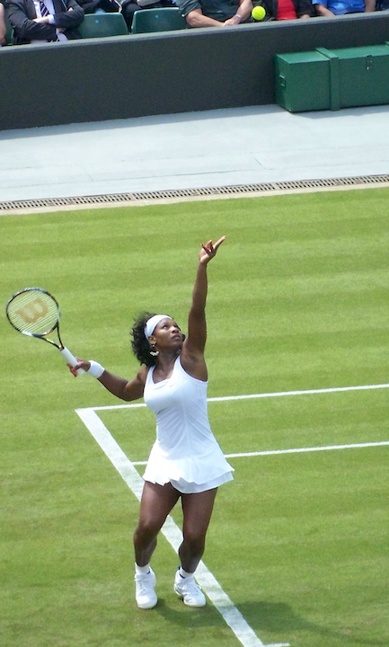
Fig. 4.6 Serena Williams serving at the 2008 Wimbledon championships [8].#
Fig. 4.6 shows Serena Williams serving during the 2008 Wimbledon championships. Williams is widely regarded as one of the best women tennis players and holds the record of most aces (scoring a point from a serve without the opponent touching the ball) by a female player at a Grand Slam tournament. Williams is 175 cm tall. As you can see in the figure, at the top of its trajectory, the ball is about twice Williams’ height above the ground. Also, as the span of people’s arms is about the same as their height, and the shoulders of an adult are at about 5/6th of their height, we can estimate Williams’ arms to be about 75 cm long and her shoulders to be at 145 cm above the ground. The distance between the point where a player holds the racket and where they hit the ball is typically about 40 cm.
Find the speed of the ball coming down at the moment Williams hits it, assuming that she hits it with a fully upward stretched arm.
Williams’s personal record for serve speed (speed of the ball after it was hit by the racket) is 207 km/h. Determine the impulse she delivered with her racket on the 58.0 g tennis ball as she hit it.
Assuming a typical racket weight of 360 g, calculate the change in speed of the racket from just before to just after Williams hit the ball.
Calculate the magnitude of the force on Williams’ hand at the moment she hits the ball with her racket.
Exercise 4.7 (A bullet and a block)
A \(2.75\;\mathrm{g}\) bullet embeds itself in a \(1.50\;\mathrm{kg}\) block, which is attached to a spring of force constant \(850\;\mathrm{N}/\mathrm{m}\). The maximum compression of the spring is \(4.30\;\mathrm{cm}\). Determine the initial speed of the bullet.
Exercise 4.8 (Head-on collision between two balls)
A ball of mass \(m\) has velocity \(v\) when it makes a head-on collision with another ball of mass \(M\) that is originally at rest. After the collision the ball of mass \(m\) rebounds straight back along its path with \(2/3^\mathrm{rd}\) of its initial kinetic energy. We assume that the collision is totally elastic.
Sketch the situation before and after the collision, indicating directions of velocity, and values (if known, give symbols otherwise).
Write down all applicable conservation laws for this case.
From the conservation laws, solve for the mass \(M\) of the ball that is initially at rest.
Also solve for the velocity of that ball after the collision.
Exercise 4.9 (Two dropping and colliding balls)
A small ball of mass \(m\) is aligned above a larger ball of mass \(M\) with a slight separation, and the two are dropped simultaneously from a height \(h\). Assume the radii of the two balls and the initial separation are negligible compared to \(h\).
If the larger ball rebounds elastically from the floor and then the small ball rebounds elastically from the larger ball, what value of \(m\) (as a fraction of \(M\)) results in the larger ball stopping when it collides with the small ball?
What height does the small ball then reach?