3. Energy

3.1. Work

How much work do you need to do to move a box? The answer depends on two things: how heavy the box is, and how far you have to move it. Multiply the two, and you’ve got a good measure of how much work will be required. Of course, work can be done in other contexts as well - pulling a spring from equilibrium, or cycling against the wind. In each case, there’s a force and a displacement. To be fair, we will only count the part of the force that is in the direction of the displacement (when cycling, you don’t do work due to the fact that there’s a gravitational force pulling you down, since you don’t move vertically; you do work because there’s a drag force due to your moving through the air). We define work as the product of the component of the force in the direction of the displacement, times the displacement itself. We calculate this component by projecting the force vector on the displacement vector, using the dot product (see Section 15.1.1 for an introduction to vector math):

(3.1)\[ W = \bm{F} \cdot \bm{x}. \]

Note that work is a scalar quantity - it has a magnitude but no direction. Work is measured in Joules (J), with one Joule being equal to one Newton times one meter.

Of course the force acting on our object need not be constant everywhere. Take for example the extension of a spring: the further you pull, the larger the force gets, as given by Hooke’s law (2.7). To calculate the work done when extending the spring, we chop up the path (here a straight line) into many small pieces. For each piece, we approximate the force by the average value on that piece, then multiply with the length of the piece and sum. In the limit that we have infinitely many pieces, this approximation becomes exact, and the sum becomes an integral: for one dimension, we thus have:

(3.2)\[ W = \int_{x_1}^{x_2} F(x) \mathrm{d}x. \]

Likewise, the path along which we move need not be a straight line. If the path consists of multiple straight segments, on each of which the force is constant, we can calculate the total work by adding the work done on the different segments. Taking the limit to infinitely many infinitesimally small segments \(\mathrm{d}\bm{r}\), on each of which the force is given by the value \(\bm{F}(\bm{r})\), the sum again becomes an integral:

(3.3)\[ W = \int_{\bm{r}_1}^{\bm{r}_2} \bm{F}(\bm{r}) \cdot \mathrm{d}\bm{r}. \]

Equation (3.3) is the most general version of the definition of work; it simplifies to (3.2) for movement along a straight line, and to (3.1) if both the path is straight and the force constant^[1].

In general, the work done depends on the path taken - for example, it’s more work to take a detour when biking from home to work, assuming the air drag is the same everywhere. However, in many important cases the work done in getting from one point to another depends on the endpoints only. Forces for which this is true are called conservative forces. As we’ll see below, the force exerted by a spring and that exerted by gravity are both conservative.

Sometimes we will not be interested in how much work is done in generating a certain displacement, but over a certain amount of time - for instance, a generator generates work by getting something to move, like a wheel or a valve, but we don’t typically care about those details, we want to know how much work we can expect to get out of the generator, i.e., how much power it has. Power is defined as the amount of work per unit time, or

(3.4)\[ P = \frac{\mathrm{d}W}{\mathrm{d}t}. \]

Power is measured in Joules per second, or Watts (W). To find out how much work is done by an engine that has a certain power output, we need to integrate that output over time:

(3.5)\[ W = \int P \mathrm{d}t. \]

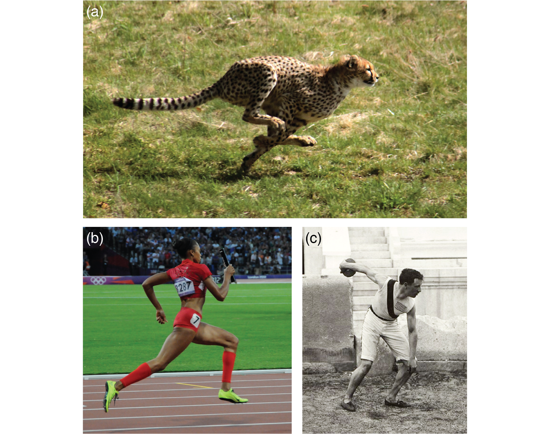
Fig. 3.1 Examples of high power resulting in high kinetic energy. (a) Running cheetah, the fastest land animal, which can reach speeds over 100 km/h in 2-3 seconds, corresponding to an enormous increase in its kinetic energy ^[2], CC BY-SA 3.0. (b) Allyson Felix running second in the women’s \(4 \times 400\) relay of the 2012 London Summer Olympics ^[3], CC BY-SA 3.0. (c) Robert Garrett preparing to throw the discus at the 1896 Athens Summer Olympics ^[4]. Unlike the runners, the goal of discus throwing is to maximize the distance, not the speed, but to get the largest possible distance, the discus must still get the maximal possible kinetic energy.

3.2. Kinetic energy

Newton’s first law told us that a moving object will stay moving unless a force is acting on it - which holds for moving with any speed, including zero. Now if you want to start moving something that is initially at rest, you’ll need to accelerate it, and Newton’s second law tells you that this requires a force - and moving something means that you’re displacing it. Therefore, there is work involved in getting something moving. We define the kinetic energy (\(K\)) of a moving object to be equal to the work required to bring the object from rest to that speed, or equivalently, from that speed to rest:

(3.6)\[ K = \frac12 m v^2. \]

Because the kinetic energy is equal to an amount of work, it is also a scalar quantity, has the same dimension, and is measured in the same unit. The factor \(v^2\) is the square of the magnitude of the velocity of the moving object, which you can calculate with the dot product: \(v^2 = \bm{v} \cdot \bm{v}\). You may wonder where equation (3.6) comes from. Newton’s second law tells us that \(\bm{F} = m \mathrm{d}\bm{v}/\mathrm{d}t\), relating the force to an infinitesimal change in the velocity. In the definition for work, equation (3.3), we multiply the force with an infinitesimal change in the position \(\mathrm{d}\bm{r}\). That infinitesimal displacement takes an infinitesimal amount of time \(\mathrm{d}t\), which is related to the displacement by the instantaneous velocity \(\bm{v}\): \(\mathrm{d}\bm{r} = \bm{v} \mathrm{d}t\). We can now calculate the work necessary to accelerate from zero to a finite speed:

(3.7)\[ K = \int \bm{F} \cdot \mathrm{d}\bm{r} = \int m \frac{\mathrm{d}\bm{v}}{\mathrm{d}t} \cdot \bm{v} \mathrm{d}t = \int m \bm{v} \cdot \frac{\mathrm{d}\bm{v}}{\mathrm{d}t} \mathrm{d}t = \int m \bm{v} \cdot \mathrm{d}\bm{v} = \frac{m}{2} \int \mathrm{d}(\bm{v} \cdot \bm{v}) = \frac12 m v^2, \]

where we used that the dot product is commutative and the fact that the integral over the derivative of a function is the function itself.

Of course, now that we know that the kinetic energy is given by equation (3.6), we no longer need to use a complicated integral to calculate it. However, because the kinetic energy is ultimately given by this integral, which is equal to a net amount of work, we arrive at the following statement, sometimes referred to as the Work-energy theorem: the change in kinetic energy of a system equals the net amount of work done on or by it (in case of increase/decrease of \(K\)):

(3.8)\[ \Delta K = W_\mathrm{net}. \]

Gabrielle Émilie Le Tonnelier de Breteuil, marquise du Châtelet (1706-1749)

Gabrielle Émilie Le Tonnelier de Breteuil, marquise du Châtelet (1706-1749), known as Émilie du Châtelet, was a French mathematician and physicist (then known as natural philosopher), who made important contributions to the development of the concept of (kinetic) energy. She translated Newton’s Principia into French, and wrote an extensive commentary on it, in which she first postulated the law of conservation of energy, for which she introduced the new concept of kinetic energy. Inspired by experiments first done by ‘s Gravesande, which she repeated and analyzed, she discovered that a ball dropped from a given height \(h\) would make an indentation in a piece of soft clay with a depth proportional to the height the ball was dropped from. At the time, most people, including Newton, considered energy to be equivalent to momentum (and thus proportional to velocity); had they been correct, the depth of the indentation should be proportional to \(\sqrt{h}\) instead. Du Châtelet’s work showed this to be incorrect, postulating instead that kinetic energy is proportional to the square of the velocity. Émilie du Châtelet was born in the French nobility, corresponded with people across Europe, married at age 18, and had a long-term friendship with Voltaire, with whom she collaborated extensively in her work on mathematics and physics. She published several books, often initially anonymously to avoid sexist prejudices, which found their way to salons and universities of the time. Her translation of the Principia is still the standard French version. She died in childbirth at age 42.

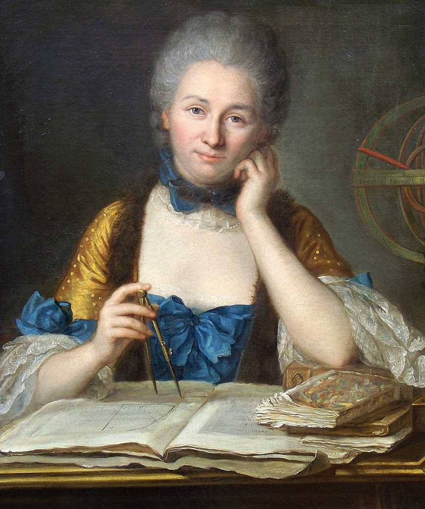
Fig. 3.2 Portrait of Émilie du Châtelet, by Maurice Quentin de La Tour ^[5].

3.3. Potential energy

We already encountered conservative forces in Section 3.1. The work done by a conservative force is (by definition) path-independent; that means that in particular the work done when moving along any closed path^[6] must be zero:

(3.9)\[ \oint \bm{F} \cdot \mathrm{d}\bm{r} = 0. \]

For a conservative force, we can thus define a potential energy difference between points 1 and 2 as the work necessary to move an object from point 1 to point 2:

(3.10)\[ \Delta U_{12} = - \int_{\bm{r}_1}^{\bm{r}_2} \bm{F} \cdot \mathrm{d}\bm{r}. \]

Note the minus sign in the definition - this is a choice of course, and you’ll see below why we made this choice. Note also that the potential energy is defined only between two points. Often we will choose a convenient reference point and calculate the potential energy at any other point with respect to that point. The reference point is typically either the origin or infinity, if the force happens to be zero at either of these. Let’s suppose we have set such a point, and know the potential energy difference with that point at any other point in space - this defines a (scalar) function \(U(\bm{r})\). If we now want to know the force acting on a particle at \(\bm{r}\), all we need to do is take the derivative of \(U(\bm{r})\) - that is to say the gradient in three dimensions (which simplifies to the ordinary derivative in one dimension):

(3.11)\[ \bm{F}(\bm{r}) = - \bm{\nabla} U(\bm{r}). \]

Equation (3.11) is extremely useful, as it gives us a means to calculate the force, which is a vector quantity, from the potential energy function, which is a scalar quantity - and therefore much simpler to work with. For instance, since energies are scalars, they can simply be added, as we’ll do in the next section, whereas for forces you need to do vector addition. Equation (3.11) also reflects that we are free to choose a reference point for the potential energy, since the force does not change if we add a constant to the potential energy.

3.3.1. Gravitational potential energy

We saw in Section 2.2.2 that for low altitudes, the gravitational force is given by \(\bm{F}_g = m \bm{g}\), where \(\bm{g}\) is a vector of constant magnitude \(g\approx 9.81 \mathrm{m}/\mathrm{s}^2\) and always points down. Therefore, the gravitational force does no work when you move horizontally, and if you first move up and then the same amount down again, it doesn’t do any net work either, as the two contributions exactly cancel. \(\bm{F}_g\) is therefore an example of a conservative force, and we can define and calculate the gravitational potential energy \(U_g\) between a point at height \(0\) (our reference point) and one at height \(h\):

(3.12)\[ U_\mathrm{g}(h) = - \int_{z=0}^{z=h} m (-g) \mathrm{d}z = m g h. \]

Note that by choosing a minus sign in the definition of the potential energy, we end up with a positive value of the energy here.

What about larger distances, i.e., Newton’s law of gravity, equation (2.9)? Well, there the distances are measured radially, so any movement perpendicular to the radial direction doesn’t matter, and if you move out and back in again, the net work done is zero, so by the same reasoning as before we again have a conservative force. This force vanishes at infinity, so it makes sense to set that as a reference point - though notice that that will make our potential energy always negative in this case:

(3.13)\[ U_\mathrm{G}(r) = - \frac{G M m}{r} \]

where \(r\) is the distance between \(m\) and \(M\), and \(M\) sits at the origin. Of course we can also calculate gravitational potential differences between two distances \(r_1\) and \(r_2\) from \(M\): \(\Delta U_\mathrm{G}(r_1, r_2) = G M m \left(\frac{1}{r_1} - \frac{1}{r_2}\right)\).

3.3.2. Spring potential energy

Like the gravitational force, the Hookean spring force (2.7) also depends on displacement alone, and by the same reasoning is conservative (notice the pattern?). Calculating its associated potential energy is straightforward, and taking the equilibrium position of the spring as the reference point, we find:

(3.14)\[ U_\mathrm{s}(x) = \frac12 k x^2. \]

The minus sign in Hooke’s Law gives us a positive spring potential energy. Note that \(x\) stands for displacement here; as we only consider one-dimensional springs the 1D-version is sufficient.

3.3.3. General conservative forces

In the case of the gravitational and spring force it was easy to reason that they had to be conservative. It is also easy to see that the friction force is not conservative: if you take a longer path, you need to do more net work against friction, which you can moreover never recover as mechanical energy. For more complicated systems, especially in three dimensions, it may not be so easy to see whether a force is conservative. Fortunately, there is an easy test you can perform: if the curl of a force is zero everywhere, it will be a conservative force, or expressed mathematically:

(3.15)\[ \bm{\nabla} \times \bm{F} = 0 \quad \Leftrightarrow \quad \oint \bm{F} \cdot \mathrm{d}\bm{r} = 0 \quad \Leftrightarrow \quad \bm{F} = - \bm{\nabla} U. \]

Is is straightforward to show that if a force is conservative, its curl must vanish: a conservative force can be written as the gradient of some scalar function \(U(\bm{x})\), and \(\bm{\nabla} \times \bm{\nabla} U(\bm{x}) = 0\) for any function \(U(\bm{x})\), as you can easily check for yourself. The proof the other way around is more complicated, and can be found in advanced mechanics textbooks.

3.4. Conservation of energy

Work, kinetic energy and potential energy are all quantities with the same dimension - so we can do arithmetic with them. One particularly useful quantity is the total energy \(E\) of a system, which is simply the sum of the kinetic and potential energy:

(3.16)\[ E = K + U. \]

Theorem 3.1 (Law of conservation of energy)

If all forces in a system are conservative, the total energy in that system is conserved.

Proof. For simplicity, we’ll look at the 1D case (3D goes analogously). Conserved means not changing in time, so in order to prove the statement, we only need to calculate the time derivative of \(E\) and check that it is always zero.

(3.17)\[\begin{split}\begin{align*} \frac{\mathrm{d}E}{\mathrm{d}t} &= \frac{\mathrm{d}K}{\mathrm{d}t} + \frac{\mathrm{d}U}{\mathrm{d}t} \\ &= \frac{\mathrm{d}\left( \frac12 m v^2 \right)}{\mathrm{d}t} + \frac{\mathrm{d}U}{\mathrm{d}x} \frac{\mathrm{d}x}{\mathrm{d}t} \\ &= m v \frac{\mathrm{d}v}{\mathrm{d}t} - F v \\ &= - \left(F - m \frac{\mathrm{d}v}{\mathrm{d}t}\right) v \\ &= 0, \end{align*}\end{split}\]

where the last equality holds because of Newton’s second law.

Conservation of energy means that the total energy of a system cannot change, but of course the potential and kinetic energy can - and by conservation of total energy we know that they get converted directly into one another. Exploiting this fact will allow us to analyze and easily solve many problems in classical mechanics - this conservation law is an immensely useful tool.

Note that conservation of energy is not the same as the work-energy theorem of Section 3.2. For the total energy to be conserved, all forces need to be conservative. In the work-energy theorem, this is not the case. You can therefore calculate changes in kinetic energy due to the work done by non-conservative forces using the latter.

3.5. Energy landscapes

In the previous section we proved that the total energy is conserved. In the section before that, we looked at potential energies. Typically, the potential energy is a function of your position in space. When we plot it as a function of spatial coordinates, we get an energy landscape, measuring an amount of energy on the vertical axis. Of course we can also plot the total energy of the system - and since that is conserved, it is the same everywhere, and thus becomes a horizontal line or plane. Because kinetic energy cannot be negative, any point where the potential energy is higher than the total energy is not allowed: the system cannot reach this point. When the potential energy equals the total energy, the kinetic energy (and thus the speed) has to be zero. Whenever the potential energy is lower than the total energy, there is a positive kinetic energy and thus a positive speed.

Probably the simplest energy landscape is that of the harmonic oscillator (mass on a spring) - it’s a simple parabola. The point at which the horizontal line representing the total energy crosses the parabola corresponds to the extrema of the oscillation: these are its turning points. The bottom of the parabola is its midpoint, and you can immediately see that that’s where the kinetic energy (and thus the speed) will be highest.

Of course you can have more complex energy landscapes than that. In particular, you can have a landscape with multiple extrema, see for example Fig. 3.3. A particle that is being acted upon by forces described by this potential energy, follows a trajectory in this landscape, which can be visualized as a ball rolling over the hills and valleys of the landscape. Think back to the harmonic oscillator example. If we let go of a ball in a parabolic vase at some point on the slope, the ball will roll down and pick up speed, then roll up the opposite slope and lose speed, until it reaches the same height where its speed will again be zero. The same is true in more complicated landscapes. Particularly interesting are local maxima. If you put a ball exactly on top of one of them, it will stay there - it is a fixed point, but an unstable one, as any arbitrarily small perturbation will push it down. If you let go of a ball at a level above a local maximum, it may hop over it to the next minimum, but if your initial position (your initial energy) was too low, your ball can get stuck oscillating about a local minimum - a metastable point.

Show code cell source Hide code cell source

import plotly.graph_objects as go
import numpy as np
from myst_nb import glue

def U(x):
    return (x**2)*(x**2 - 2)*(x + 1)*(x - 2)

def dU(x):
    return x*(6*x**4 - 5*x**3 - 16*x**2 + 6*x + 8)  # Derivative of U(x)

x = np.linspace(-2, 2.5, 100)
y = U(x)

fig = go.Figure(layout=go.Layout(template='simple_white'))
#fig = go.Figure()

# Have hover text for each point on function U(x) be equal to U'(x).
dU_values = dU(x)
hover_texts = [f'<i>U</i>\'(<i>x</i>) = {val:.3f}' for val in dU_values]

# Add function trace for potential energy U(x)
function_trace = go.Scatter(
    x=x, 
    y=y, 
    mode='lines', 
    name='Potential energy function', 
    #line=dict(color='blue'),
    legendgroup='function',  # Assign to its own legend group so it is always visible and non-toggleable from the legend
    showlegend=False,  # Hide from legend
    text=hover_texts,  # Set the hover text for each point
    hoverinfo='text'  # Display only the hover text
)
fig.add_trace(function_trace)


# Add equilibrium points
extreme_x = {
    'Unstable equilibria': [-0.635, 0.942],  # Local max
    'Metastable equilibria': [-1.254, 0],  # Local min
    'Globally stable equilibrium': [1.779]  # Global min
}
extreme_y = {etype: [U(x_val) for x_val in x_values] for etype, x_values in extreme_x.items()}

extrema_traces = []
for etype, color in [
    ('Unstable equilibria', 'green'), 
    ('Metastable equilibria', 'orange'), 
    ('Globally stable equilibrium', 'red')]:
    extremum_dict = {'Unstable equilibria': 'Local maximum', 'Metastable equilibria': 'Local minimum', 'Globally stable equilibrium': 'Global minimum'}
    hover_text = f'<i>U</i>\'(<i>x</i>) = 0\n{extremum_dict[etype]}'
    trace = go.Scatter(
        x=extreme_x[etype], 
        y=extreme_y[etype], 
        mode='markers', 
        name=f'{etype}', 
        marker=dict(color=color, size=10),
		text=hover_text,
        hoverinfo='text'
    )
    fig.add_trace(trace)
    extrema_traces.append(trace)

fig.update_layout(
    #title_text='A potential energy landscape and its equilibrium points', 
    #title_x=0.5, 
    showlegend=True,
    yaxis=dict(range=[-3, 4]),
    xaxis_title='<i>x</i>',
    yaxis_title='<i>U</i>(<i>x</i>)',
	xaxis_title_font = dict(size=24, family='Times New Roman'),
	yaxis_title_font = dict(size=24, family='Times New Roman')
)

# fig.show()

# Save graph to load in figure later (special Jupyter Book feature)
glue("InteractiveEnergyLandscape", fig, display=False)

Fig. 3.3 An example of a potential energy landscape. In this figure, the total energy would be represented by a horizontal line; the kinetic energy by the distance between the potential and total energy. Equlibrium points (dots) occur at extrema of the potential energy, when its derivative (the force) is zero. The green dots indicate unstable equilibrium points (maxima, where the second derivative is negative), the orange points metastable equilibria (local minima) and the red point the single globally stable equilibrium of this system.

Energy landscapes are even useful when the total energy is not conserved - for example because of friction terms. Friction causes energy to dissipate from the system, which is equivalent to having your ball move in the landscape with friction. For low friction, your ball will oscillate, but get less high every time, until it comes to rest at the minimum. For high friction, it won’t even oscillate, but just get to the minimum - exactly what an overdamped system in real life does.

Show code cell source Hide code cell source

%config InlineBackend.figure_formats = ['svg']
import numpy as np
import matplotlib.pyplot as plt
plt.rcParams.update({'font.size': 16})
from myst_nb import glue

def U(r):
	# Returns U(r), in units where sigma = 1 and epsilon = 1.
	return 4 * (np.power(r, -12) - np.power(r, -6))

# Define r_eq, in units where sigma = 1 and epsilon = 1.
req = np.power(2, 1/6)

fig, ax = plt.subplots(figsize=(6,4))

r = np.linspace(0.01, 3, 299)

line1 = ax.plot(r, U(r), linewidth=3)

ax.axhline(y=0, color='k', linestyle='--')

# Lines to plot from v-axis and U-axis.
ax.plot([req, req], [0, U(req)], color='k', linestyle = ':')
ax.plot([0, req], [U(req), U(req)], color='k', linestyle = ':')

# Point at r_eq.
ax.plot(req, 0, 'o')

# Label the point.
ax.text(req, 0.2, '$r_\\mathrm{eq} = 2^{1/6} \\sigma$', color='C1', horizontalalignment='left')

# Axis settings
ax.set_xlim(0, 2.7)
ax.set_ylim(-1.2,4.2)
ax.set_xlabel('$r/\\sigma$')
ax.set_ylabel('$U/\\varepsilon$')

# Save graph to load in figure later (special Jupyter Book feature)
glue("LennardJones", fig, display=False)

Example 3.1 (The Lennard-Jones potential)

The Lennard-Jones potential energy is a commonly used model to describe the interactions between uncharged atoms and molecules. This potential energy can be written in two equivalent ways:

(3.18)\[U_\mathrm{LJ}(r) = \frac{A}{r^{12}} - \frac{B}{r^6} = 4 \varepsilon \left[ \left(\frac{\sigma}{r}\right)^{12} - \left(\frac{\sigma}{r}\right)^6 \right],\]

where \(r\) is the distance between the atoms or molecules, and \(A\), \(B\), \(\varepsilon\) and \(\sigma\) are positive constants.

1. Find the dimensions of \(A\), \(B\), \(\varepsilon\) and \(\sigma\).

2. Express \(\varepsilon\) and \(\sigma\) in \(A\) and \(B\).

3. Sketch the potential (in its second form) as a function of \(r/\sigma\), and use this sketch to give a physical interpretation of \(\varepsilon\) and \(\sigma\).

4. Does the Lennard-Jones potential lead to attractive or repulsive forces at short distances? And what about long distances?

5. Find all equilibrium points of this potential energy, and determine their stability.

---

Solution

1. \([U]= \text{Energy} \Longrightarrow [U] = M \times \frac{L}{T^2} \times L = \frac{ML^2}{T^2}\) \([A]= \text{Energy} \times \text{Length}^{12} \Longrightarrow [A]=\frac{ML^{14}}{T^2} \) \([B]= \text{Energy} \times \text{Length}^{6} \Longrightarrow [A]=\frac{ML^{8}}{T^2} \) The powers of the terms \(\left(\frac{\sigma}{r}\right)^{12}\) and \(\left(\frac{\sigma}{r}\right)^6\) are different, but in the potential energy, we subtract them. The only way we can do so is if they are dimensionless. Thus, \([\sigma]=L\) and \([\varepsilon]=[U]=\frac{ML^2}{T^2}\).

2. We can simply read off that

   \[\begin{split}\begin{align*} & 4\epsilon \sigma ^{12} = A \text{ and } 4\varepsilon \sigma^{6} = B\\ & \frac{A}{B} = \sigma^6 \Longrightarrow \sigma= \left(\frac{A}{B}\right)^{1/6}. \end{align*}\end{split}\]

   By substituting \(\sigma\) in the expressions for either \(A\) or \(B\) we can derive an expression for \(\varepsilon\):

   \[\begin{split}\begin{align*} 4\sigma^6 \varepsilon &= B \\ 4 \varepsilon A &= B^2 \Longrightarrow \varepsilon = \frac{B^2}{4A}. \end{align*}\end{split}\]

3. See Fig. 3.4. Interpretation: \(\epsilon\) is a measure for the depth of the potential well. \(\sigma\) sets the length scale and therefore the position of the equilibrium point.

   

   Fig. 3.4 Sketch of the Lennard-Jones potential energy.

4. Method 1: We calculate the force as minus the derivative of the potential energy:

   \[\begin{align*} F = -\frac{\partial U}{\partial r} = 4 \varepsilon \left(\frac{12 \sigma^{12}}{r^{13}}-\frac{6 \sigma^{6}}{r^{7}} \right) \end{align*}\]

   For small \(r\) we have \(r^{-13} \gg r^{-7}\), so \(F\) is positive and therefore repulsive. Conversely, for large \(r\) we have \(r^{-13} \ll r^{-7}\), so \(F\) is negative and therefore attractive.

   Method 2: Use the sketch in (c) to to see that the slope of the potential is negative for small \(r\), which implies a repulsive force, and the slope of the potential is positive for large \(r\), which implies an attractive force.

5. For an equilibrium point we have:

   \[0 = \frac{\partial U}{\partial r} = 4 \varepsilon \left(\frac{12 \sigma^{12}}{r^{13}}-\frac{6 \sigma^{6}}{r^{7}} \right) = 24 \frac{\varepsilon\sigma^6}{r^7} \left(\frac{2 \sigma^{6}}{r^{6}}-1 \right),\]

   so there is only one equilibrium point, at

   \[r_\mathrm{eq} = 2^{1/6}\sigma.\]

   To determine the stability at this point, we consider the second derivative of \(U(r)\):

   \[\begin{split}\begin{align*} \left. \frac{\partial^2U}{\partial r^2}\right|_{r = r_\mathrm{eq}} \!\! &= 4 \varepsilon \left. \left(42 \frac{\sigma^6}{r^8} - 156 \frac{\sigma^{12}}{r^{14}} \right)\right|_{r = r_\mathrm{eq}} \!\! = 4 \varepsilon \left( \frac{42}{2^{4/3} \sigma^2} - \frac{156}{2^{7/3} \sigma^2}\right) \\ &= - 36 \cdot 2^{2/3} \frac{\varepsilon}{\sigma^2} < 0, \end{align*}\end{split}\]

   which means that the equilibrium point is stable. Alternatively, we could have determined the stability by considering the graph drawn at (c), from which we can see that the equilibrium point corresponds to a global minimum of the potential energy and hence is stable.

3.6. Problems

Exercise 3.1 (Firing a cannon ball)

1. Show that, if you ignore drag, a projectile fired at an initial velocity \(v_0\) and angle \(\theta\) has a range \(R\) given by

   (3.19)\[R = \frac{v_0^2 \sin 2\theta}{g}.\]

2. A target is situated 1.5 km away from a cannon across a flat field. Will the target be hit if the firing angle is \(42^\circ\) and the cannonball is fired at an initial velocity of \(121\;\mathrm{m}/\mathrm{s}\)? (Cannonballs, as you know, do not bounce).

3. To increase the cannon’s range, you put it on a tower of height \(h_0\). Find the maximum range in this case, as a function of the firing angle and velocity, assuming the land around is still flat.

Exercise 3.2 (Pushing a box uphill)

You push a box of mass \(m\) up a slope with angle \(\theta\) and kinetic friction coefficient \(\mu\). Find the minimum initial speed \(v\) you must give the box so that it reaches a height \(h\).

Exercise 3.3 (Work done dragging a board)

A uniform board of length \(L\) and mass \(M\) lies near a boundary that separates two regions. In region 1, the coefficient of kinetic friction between the board and the surface is \(\mu_1\), and in region 2, the coefficient is \(\mu_2\). Our objective is to find the net work \(W\) done by friction in pulling the board directly from region 1 to region 2, under the assumption that the board moves at constant velocity.

1. Suppose that at some point during the process, the right edge of the board is a distance \(x\) from the boundary, as shown. When the board is at this position, what is the magnitude of the force of friction acting on the board, assuming that it’s moving to the right? Express your answer in terms of all relevant variables (\(L\), \(M\), \(g\), \(x\), \(\mu_1\), and \(\mu_2\)).

2. As we’ve seen in Section 3.1, when the force is not constant, you can determine the work by integrating the force over the displacement, \(W = \int F(x) \mathrm{d}x\). Integrate your answer from (a) to get the net work you need to do to pull the board from region 1 to region 2.

Exercise 3.4 (Highway speed limits)

The government wishes to secure votes from car-owners by increasing the speed limit on the highway from \(120\) to \(140\;\mathrm{km}/\mathrm{h}\). The opposition points out that this is both more dangerous and will cause more pollution. Lobbyists from the car industry tell the government not to worry: the drag coefficients of the cars have gone down significantly and their construction is a lot more solid than in the time that the \(120\;\mathrm{km}/\mathrm{h}\) speed limit was set.

1. Suppose the \(120\;\mathrm{km}/\mathrm{h}\) limit was set with a Volkswagen Beetle (\(c_d = 0.48\)) in mind, and the lobbyist’s car has a drag coefficient of \(0.19\). Will the new car need to do more or less work to maintain a constant speed of \(140\;\mathrm{km}/\mathrm{h}\) than the Beetle at \(120\;\mathrm{km}/\mathrm{h}\)?

2. What is the ratio of the total kinetic energy released in a full head-on collision (resulting in an immediate standstill) between two cars both at \(140\;\mathrm{km}/\mathrm{h}\) and two cars both at \(120\;\mathrm{km}/\mathrm{h}\)?

3. The government dismisses the opposition’s objections on safety by stating that on the highway, all cars move in the same direction (opposite direction lanes are well separated), so if they all move at \(140\;\mathrm{km}/\mathrm{h}\), it would be just as safe as all at \(120\;\mathrm{km}/\mathrm{h}\). The opposition then points out that running a Beetle (those are still around) at \(120\;\mathrm{km}/\mathrm{h}\) is already challenging, so there would be speed differences between newer and older cars. The government claims that the \(20\;\mathrm{km}/\mathrm{h}\) difference won’t matter, as clearly even a Beetle can survive a \(20\;\mathrm{km}/\mathrm{h}\) collision. Explain why their argument is invalid.

Exercise 3.5 (Nuclear fusion)

Nuclear fusion, the process that powers the Sun, occurs when two low-mass atomic nuclei fuse together to make a larger nucleus, releasing substantial energy. Fusion is hard to achieve because atomic nuclei carry positive electric charge, and their electrical repulsion makes it difficult to get them close enough for the short-range nuclear force to bind them into a single nucleus. The figure below shows the potential-energy curve for fusion of two deuterons (heavy hydrogen nuclei, consisting of a proton and a neutron). The energy is measured in million electron volts (MeV, \(1\;\mathrm{eV} = 1.6 \cdot 10^{-19}\;\mathrm{J}\)), a unit commonly used in nuclear physics, and the separation is in femtometers (\(1\;\mathrm{fm} = 10^{-15}\;\mathrm{m}\)).

1. Find the position(s) (if any) at which the force between two deuterons is zero.

2. Find the kinetic energy two initially widely separated deuterons need to have to get close enough to fuse.

3. The energy available in fusion is the energy difference between that of widely separated deuterons and the bound deutrons after they’ve ‘fallen’ into the deep potential well shown in the figure. About how big is that energy?

4. Determine whether the force between two deuterons that are \(4\;\mathrm{fm}\) apart is repulsive, attractive, or zero.

Exercise 3.6 (Flying pigeon)

A pigeon in flight experiences a drag force due to air resistance given approximately by \(F = bv^2\), where \(v\) is the flight speed and \(b\) is a constant.

1. What are the units of \(b\)?

2. What is the largest possible speed of the pigeon if its maximum power output is \(P\)?

3. By what factor does the largest possible speed increase if the maximum power output is doubled?

Exercise 3.7 (Conservative forces)

1. For which value(s) of the parameters \(\alpha\), \(\beta\) and \(\gamma\) is the force given by

   \[\bm{F} = (x^3 y^3 + \alpha z^2, \beta x^4 y^2, \gamma x z)\]

   conservative?

2. Find the force for the potential energy given by \(U(x, y, z) = x y / z - x z / y\).

Exercise 3.8 (A point mass connected by two springs)

A point mass is connected to two opposite walls by two springs, as shown in the figure. The distance between the walls is \(2L\). The left spring has rest length \(l_1 = L/2\) and spring constant \(k_1 = k\), the right spring has rest length \(l_2 = 3L/4\) and spring constant \(k_2 = 3k\).

1. Determine the magnitude of the force acting on the point mass if it is at \(x=0\).

2. Determine the equilibrium position of the point mass.

3. Find the potential energy of the point mass as a function of \(x\). Use the equilibrium point from (b) as your point of reference.

4. If the point mass is displaced a small distance from its equilibrium position and then released, it will oscillate. By comparing the equation of the net force on the mass in this system with a simple harmonic oscillator, determine the frequency of that oscillation. (We’ll return to systems oscillating about the minimum of a potential energy in Section 8.1.4, feel free to take a sneak peak ahead).

Exercise 3.9 (A block hitting a spring)

A block of mass \(m = 3.50\;kg\) slides from rest a distance \(d\) down a frictionless incline at angle \(\theta = 30.0^\circ\), where it runs into a spring of spring constant \(450\;\mathrm{N}/\mathrm{m}\). When the block momentarily stops, it has compressed the spring by \(25.0\;\mathrm{cm}\).

1. Find \(d\).

2. What is the distance between the first block-spring contact and the point at which the block’s speed is greatest?

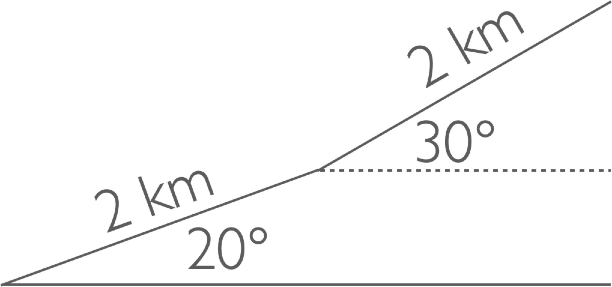
Exercise 3.10 (Sliding down a playground slide)

Playground slides frequently have sections of varying slope: steeper ones to pick up speed, less steep ones to lose speed, so kids (and students) arrive at the bottom safely. We consider a slide with two steep sections (angle \(\alpha\)) and two less steep ones (angle \(\beta\)). Each of the sections has a width \(L\). The slide has a coefficient of kinetic friction \(\mu\).

1. Kids start at the top of the slide with velocity zero. Calculate the velocity of a kid of mass \(m\) at the end of the first steep section.

2. Now calculate the velocity of the kid at the bottom of the entire slide.

3. If \(L=1.0\;\mathrm{m}\), \(\alpha = 30^\circ\) and \(\mu = 0.5\), find the minimum value \(\beta\) must have so that kids up to 30 kg can enjoy the slide (Hint: what is the minimum requirement for the slide to be functional)?

4. A given slide has \(\alpha = 30^\circ\), \(\beta = 25^\circ\) and \(\mu = 0.5\). A young child of \(10\;\mathrm{kg}\) slides down, and continues sliding on the ground after reaching the bottom of the slide. The coefficient of kinetic friction with the ground is \(0.70\). How far does the child slide before it comes to a full stop?

Exercise 3.11 (Anharmonic potential)

In this problem, we consider the anharmonic potential given by

(3.20)\[U(x) = \frac{a}{2} (x-x_0)^2 + \frac{b}{3} (x-x_0)^3,\]

where \(a\), \(b\) and \(x_0\) are positive constants.

1. Find the dimensions of \(a\), \(b\) and \(x_0\).

2. Determine whether the force on a particle at a position \(x \gg x_0\) is attractive or repulsive (taking the origin as your point of reference).

3. Find the equilibrium point(s) (if any) of this potential, and determine their stability.

4. For \(b=0\), the potential given in equation (3.20) becomes harmonic (i.e., the potential of a harmonic oscillator), in which case a particle that is initially located at a non-equilibrium point will oscillate. Are there initial values for \(x\) for which a particle in this anharmonic potential will oscillate? If so, find them, and find the approximate oscillation frequency; if not, explain why not. (NB: As the problem involves a third order polynomial function, you may find yourself having to solve a third order problem. When that happens, for your answer you can simply say: the solution \(x\) to the problem \(X\)).

Exercise 3.12 (Launching a book into orbit)

After you have successfully finished your mechanics course, you decide to launch the book into an orbit around the Earth. However, the teacher is not convinced that you do not need it anymore and asks the following question: What is the ratio between the kinetic energy and the potential energy of the book in its orbit? Let \(m\) be the mass of the book, \(M_\oplus\) and \(R_\oplus\) the mass and the radius of the Earth respectively. The gravitational pull at distance \(r\) from the center is given by Newton’s law of gravitation (equation (2.9)):

\[\bm{F}_\mathrm{g}(r) = -G \frac{mM_\oplus}{r^2} \bm{\hat{r}}\]

1. Find the orbital velocity \(v\) of an object at height \(h\) above the surface of the Earth.

2. Express the work required to get the book at height \(h\).

3. Calculate the ratio between the kinetic and the potential energy of the book in its orbit.1. What requires more work, getting the book to the International Space Station (orbiting at \(h=400\;\mathrm{km}\)) or giving it the same speed as the ISS?

Exercise 3.13 (Escape velocity)

Using dimensional arguments, in Exercise 1.4 we found the scaling relation of the escape velocity (the minimal initial velocity an object must have to escape the gravitational pull of the planet/moon/other object it’s on completely) with the mass of the radius of the planet. Here, we’ll re-derive the result, including the numerical factor that dimensional arguments cannot give us.

1. Derive the expression of the gravitational potential energy, \(U_\mathrm{g}\), of an object of mass \(m\) due to a gravitational force \(F_\mathrm{g}\) given by Newton’s law of gravitation (equation (2.9)):

   \[\bm{F}_\mathrm{g} = - \frac{G m M}{r^2} \bm{\hat{r}}.\]

   Set the value of the integration constant by \(U_\mathrm{g} \to 0\) as \(r \to \infty\).

2. Find the escape velocity on the surface of a planet of mass \(M\) and radius \(R\) by equating the initial kinetic energy of your object (when launched from the surface of the planet) to the total gravitational potential energy it has there.

Exercise 3.14 (Firing at the Moon)

A cannonball is fired upwards from the surface of the Earth with just enough speed such that it reaches the Moon. Find the speed of the cannonball as it crashes on the Moon’s surface, taking the gravity of both the Earth and the Moon into account. Table 16.3 contains the necessary astronomical data.

Exercise 3.15 (Turkish bow)

The draw force \(F(x)\) of a Turkish bow as a function of the bowstring displacement \(x\) (for \(x < 0\)) is approximately given by a quadrant of the ellipse

\[\left( \frac{F(x)}{F_{\max}}\right)^2 + \left(\frac{x+d}{d}\right)^2 = 1.\]

In rest, the bowstring is at \(x=0\); when pulled all the way back, it’s at \(x = -d\).

1. Calculate the work done by the bow in accelerating an arrow of mass \(m = 37\;\mathrm{g}\), for \(d = 0.85\;\mathrm{m}\) and \(F_{\max} = 360\;\mathrm{N}\).

2. Assuming that all of the work is converted to kinetic energy of the arrow, find the maximum distance the arrow can fly. Hint: which variable can you control when shooting? Maximize the distance with respect to that variable.

3. Compare the result of (b) with the range of a bow that acts like a simple (Hookean) spring with the same values of \(F_{\max}\) and \(d\). How much further does the arrow shot from the Turkish bow fly than that of the simple spring bow?

Exercise 3.16 (Mounted cylinder)

A massive cylinder with mass \(M\) and radius \(R\) is connected to a wall by a spring at its center (see figure). The cylinder can roll back-and-forth without slipping.

1. Determine the total energy of the system consisting of the cylinder and the spring.

2. Differentiate the energy of problem (a) to obtain the equation of motion of the cylinder and spring system.

3. Find the oscillation frequency of the cylinder by comparing the equation of motion at (b) with that of a simple harmonic oscillator (a mass-spring system).

Exercise 3.17 (Sliding off a spherical mount)

A small particle (blue dot) is placed atop the center of a hemispherical mount of ice of radius R (see figure). It slides down the side of the mount with negligible initial speed. Assuming no friction between the ice and the particle, find the height at which the particle loses contact with the ice.

Hint: To solve this problem, first draw a free body diagram, and combine what you know of energy and forces.

Exercise 3.18 (Pulling membrane tubes)

Pulling membrane tubes The (potential) energy of a cylindrical membrane tube of length \(L\) and radius \(R\) is given by

\[\mathcal{E}_\mathrm{tube}(R, L) = 2 \pi R L \left( \frac{\kappa}{2}\frac{1}{R^2} + \sigma \right).\]

Here \(\kappa\) is the membrane’s bending modulus and \(\sigma\) its surface tension.

1. Find the dimensions of the bending modulus and the surface tension.

2. Find the forces acting on the tube along its radial and axial direction.

3. Membrane tubes are often pulled by membrane motors pulling along the axial direction, as sketched in Fig. 3.5. For that case, we add the work done by the motors to the total energy of the tube, so we get:

   \[\mathcal{E}_\mathrm{tube}(R, L) = 2 \pi R L \left( \frac{\kappa}{2}\frac{1}{R^2} + \sigma \right) - F L.\]

   Show that for a stable tube, the motors need to exert a force of magnitude \(F = 2 \pi \sqrt{2\kappa \sigma}\).

4. Can the force of (c) be considered to be an effective spring force? If so, find its associated spring constant. If not, explain why not.

   

   Fig. 3.5 Cartoon of molecular motors together pulling a membrane tube.

---

[1]

If you feel intimidated by the vector form of equation (3.3), it may help to rewrite it in terms of the magnitudes of the force \(\bm{F}(\bm{r})\), the (infinitesimal) displacement \(\mathrm{d}\bm{r}\), and the angle \(\theta\) between them. In terms of \(F = |\bm{F}|\), \(\mathrm{d}r = |\mathrm{d}\bm{r}|\) and \(\theta\), we have \(\bm{F} \cdot \mathrm{d}\bm{r} = F \cos\theta \, \mathrm{d}r\), an expression you may have seen before for a force not pointing in the same direction as the displacement. If we now make the force and displacements functions of the position \(\bm{r}\), then the magnitude of the force and the angle likewise become functions of \(\bm{r}\), so we can also write equation (3.3) as

(3.21)\[W = \int_{\bm{r}_1}^{\bm{r}_2} F(\bm{r}) \cos \theta(\bm{r}) \cdot \mathrm{d}r.\]

[2]

Image by Malene Thyssen, Wikimedia commons, CC BY-SA 3.0.

[3]

Photograph of Allyson Felix at the 2012 Summer Olympics by Citizen59, Wikimedia commons, CC BY-SA 3.0.

[4]

Photograph of Robert Garrett throwing the discus at the 1896 Summer Olympics; picture by Albert Meyer, shared by the Bulgarian Archives State Agency (file BASA-3K-7-422-22) through Wikimedia commons, public domain.

[5]

Portrait of madame du Châtelet at her desk (detail), by Maurice Quentin de La Tour (early 18th century). Picture is a faithful reproduction of a two-dimensional public domain work, retrieved from Wikimedia commons.

[6]

The integral sign with the circle in equation (3.9) represents an integral over a closed path.