
5. Rotational motion, torque and angular momentum#
5.1. Rotation basics#
So far, we’ve been looking at motion that is easily described in Cartesian coordinates, often moving along straight lines. Such kind of motion happens a lot, but there is a second common class as well: rotational motion. It won’t come as a surprise that to describe rotational motion, polar coordinates (or their 3D counterparts the cylindrical and spherical coordinates) are much handier than Cartesian ones[1]. For example, if we consider the case of a disk rotating with a uniform velocity around its center, the easiest way to do so is to specify over how many degrees (or radians) a point on the boundary advances per second. Compare this to linear motion - that is specified by how many meters you advance in the linear direction per second, which is the speed (with dimension \(L/T\)). The change of the angle per second gives you the angular speed \(\omega\), where a counterclockwise rotation is taken to be in the positive direction. The angular speed has dimension \(1/T\), so it is a frequency. It is measured in degrees per second or radians per second. If the angle at a point in time is denoted by \(\theta(t)\), then obviously \(\omega = \dot{\theta}\), just like \(v = \dot{x}\) in linear motion.
In three dimensions, \(\bm{\omega}\) becomes a vector, where the magnitude is still the rotational speed, and the direction gives you the direction of the rotation, by means of a right-hand rule: rotation is in the plane perpendicular to \(\bm{\omega}\), and in the direction the fingers of your right hand point if your thumb points along \(\bm{\omega}\) (this gives \(\bm{\omega}\) in the positive \(\bm{\hat{z}}\) direction for rotational motion in the \(xy\) plane).
Going back to 2D for the moment, let’s call the angular position \(\theta(t)\), then
If we want to know the position \(\bm{r}\) in Cartesian coordinates, we can simply use the normal conversion from polar to Cartesian coordinates, and write
where \(r\) is the distance to the origin. Note that \(\bm{r}\) points in the direction of the polar unit vector \(\bm{\hat{r}}\). Equation (5.2) gives us an interpretation of \(\omega\) as a frequency: if we consider an object undergoing uniform rotation (i.e., constant radius and constant velocity), in its \(x\) and \(y\)-directions it oscillates with frequency \(\omega\).
As long as our motion remains purely rotational, the radial distance \(r\) does not change, and we can find the linear velocity by taking the time derivative of (5.2):
so in particular we have \(v=\omega r\). Note that both \(v\) and \(\omega\) denote instantaneous speeds, and equation (5.2) only holds when \(\omega\) is constant. However, the relation \(v=\omega r\) always holds. To see that this is true, express \(\theta\) in radians, \(\theta=s/r\), where \(s\) is the distance traveled along the rotation direction. Then
In three dimensions, we find
where \(\bm{r}\) points from the rotation axis to the rotating point.
Unlike in linear motion, in rotational motion there is always acceleration, even if the rotational velocity \(\omega\) is constant. This acceleration originates in the fact that the direction of the (linear) velocity always changes as points revolve around the center, even if its magnitude, the net linear speed, is constant. In that special case, taking another derivative gives us the linear acceleration, which points towards the center of rotation:
In Section 5.2 below we will use equation (5.6) in combination with Newton’s second law of motion to calculate the net centripetal force required to maintain rotation at a constant rate.
Of course the angular velocity \(\omega\) need not be constant at all. If it is not, we can define an angular acceleration by taking its time derivative:
or in three dimensions, where \(\bm{\omega}\) is a vector:
Note that when \(\bm{\alpha}\) is parallel to \(\bm{\omega}\), it simply represents a change in the rotation rate (i.e., a speeding up/slowing down of the rotation), but when it is not, it also represents a change of the plane of rotation.
In both two and three dimensions, a change in rotation rate causes the linear acceleration to have a component in the tangential direction in addition to the radial acceleration (5.6). The tangential component of the acceleration is given by the derivative of the linear velocity:
In two dimensions, \(\bm{a}_\mathrm{t}\) points along the \(\pm\bm{\hat{\theta}}\) direction.
Naturally, there are even more complicated possibilities - the radius of the rotational motion can change as well. We’ll look at that case in more detail in Section 6, but first we consider ‘pure’ rotations, where the distance to the rotation axis is fixed.
5.2. Centripetal force#
When you’re rotating at constant angular velocity, the magnitude of your velocity is always the same, but its direction constantly changes - so you’re constantly undergoing an acceleration, as indicated in equation (5.6). Therefore there must be a net force acting on you. We can calculate that net force using Newton’s second law of motion. It is known as the centripetal force and given by:
‘Centripetal’ means ‘center-seeking’ (from Latin ‘centrum’ = center and ‘petere’ = to seek). It is important to remember that this is a net resulting force, not a ‘new’ force like that exerted by gravity or a compressed spring. Equation (5.10) is after all just a special case of Newton’s second law of motion.
5.3. Torque#
Anyone who has ever used a lever - that is everyone, presumably - knows how useful they are at augmenting force: you push with a small force at the long end, to produce a large force at the short end, and make the crank turn, stone lift or bottle cap pop off. If the force is at straight angles with the lever arm (the line connecting the point at which you exert the force to the pivot around which your lever rotates), the effect is largest. In that case we define the torque (or moment of force) \(\tau\) as the product of the force and the lever arm length. As only the perpendicular component of the force counts (you’ll simply push or pull on your lever with a parallel component, not make it turn), in a vector setting you need to project on that perpendicular component, so if \(\bm{r}\) (from the pivot to the point at which the force acts) makes an angle \(\theta\) with the force vector \(\bm{F}\), the magnitude of the torque becomes \(\tau = r F \sin\theta\). That’s exactly the magnitude of the cross product of \(\bm{r}\) and \(\bm{F}\), which also has directional information - useful as a torque can be clockwise or counterclockwise. In general we’ll therefore define the torque by:
which makes a counterclockwise torque positive, in correspondence with the definition of the rotation vector \(\bm{\omega}\).
5.4. Moment of inertia#
Suppose we have a mass \(m\) at the end of a massless stick of length \(r\), rotating around the other end of the stick. If we want to increase the rotation rate, we need to apply a tangential acceleration \(\bm{a}_\mathrm{t} = r \bm{\alpha}\), for which by Newton’s second law of motion we need a force \(\bm{F} = m \bm{a}_\mathrm{t} = m r \bm{\alpha}\). This force in turn generates a torque of magnitude \(\tau = r \cdot F = m r^2 \alpha\). The last equality is reminiscent of Newton’s second law of motion, but with force replaced by torque, acceleration by angular acceleration, and mass by the quantity \(m r^2\). In analog with mass representing the inertia of a body undergoing linear acceleration, we’ll identify this quantity as the inertia of a body undergoing rotational acceleration, which we’ll call the moment of inertia and denote by \(I\):
Equation (5.12) is the rotational analog of Newton’s second law of motion. By extending our previous example, we can find the moment of inertia of an arbitrary collection of particles of masses \(m_\alpha\) and distances to the rotation axis \(r_\alpha\) (where \(\alpha\) runs over all particles), and write:
which like the center of mass in Section 4.1 easily generalizes to continuous objects as[2]
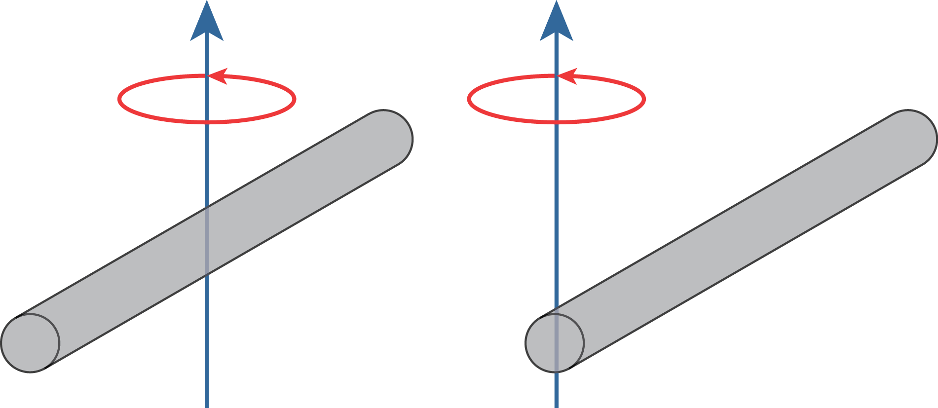
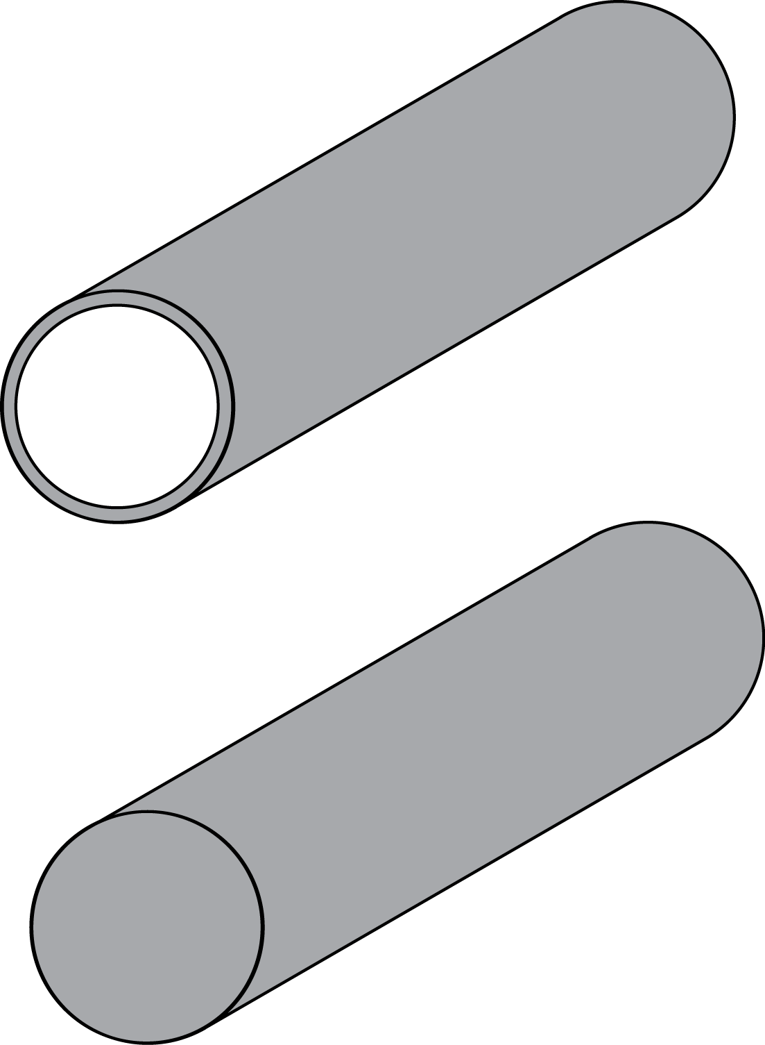
Note that it matters where we choose the rotation axis. For example, the moment of inertia of a rod of length \(L\) and mass \(m\) around an axis through its center perpendicular to the rod is \(\frac{1}{12}mL^2\), whereas the moment of inertia around an axis perpendicular to the rod but located at one of its ends is \(\frac{1}{3}m L^2\). Also, moments of inertia are different for hollow and solid objects - a hollow sphere of mass \(m\) and radius \(R\) has \(\frac23 m R^2\) whereas a solid sphere has \(\frac25 m R^2\), and for hollow and solid cylinders (or hoops and disks) around the long axis through the center we find \(m r^2\) and \(\frac14 m r^2\) respectively. These and some other examples are listed in Table 5.1. Below we’ll relate the moment of inertia to the kinetic energy of a moving-and-rolling object, but first we present two handy theorems that will help in calculating them.
Object |
Rotation axis |
Moment of inertia |
|---|---|---|
Stick |
Center, perpendicular to stick |
\(\frac{1}{12} M L^2\) |
Stick |
End, perpendicular to stick |
\(\frac{1}{3} M L^2\) |
Cylinder, hollow |
Center, parallel to axis |
\(M R^2\) |
Cylinder, solid |
Center, parallel to axis |
\(\frac12 M R^2\) |
Sphere, hollow |
Any axis through center |
\(\frac23 M R^2\) |
Sphere, solid |
Any axis through center |
\(\frac25 M R^2\) |
Planar object, size \(a \times b\) |
Axis through center, in plane, |
\(\frac{1}{12} M b^2\) |
parallel to side with length \(a\) |
||
Planar object, size \(a \times b\) |
Axis through center, |
\(\frac{1}{12} M (a^2 + b^2)\) |
perpendicular to plane |
Theorem 5.1 (Parallel axis theorem)
If the moment of inertia of a rigid body about an axis through its center of mass is given by \(I_\mathrm{cm}\), then the moment of inertia around an axis parallel to the original axis and separated from it by a distance \(d\) is given by
where \(m\) is the object’s mass.
Proof. Choose coordinates such that the center of mass is at the origin, and the original axis coincides with the \(\bm{\hat{z}}\) axis. Denote the position of the point in the \(xy\) plane through which the new axis passes by \(\mathbf{d}\), and the distance from that point for any other point in space by \(\mathbf{r}_d\), such that \(\mathbf{r} = \mathbf{d} + \mathbf{r}_d\). Now calculate the moment of inertia about the new axis through \(\mathbf{d}\):
Here \(d^2 = \mathbf{d}\cdot\mathbf{d}\). The last integral in the last line of (5.16) is equal to the position of the center of mass, which we chose to be at the origin, so the last term vanishes, and we arrive at (5.15).
Note that the first two lines of Table 5.1 (moments of inertia of a stick) satisfy the perpendicular-axis theorem.
Theorem 5.2 (Perpendicular axis theorem)
If a rigid object lies entirely in a plane, and the moments of inertia around two perpendicular axes \(x\) and \(y\) in that plane are \(I_x\) and \(I_y\), respectively, then the moment of inertia around the axis \(z\) perpendicular to the plane and passing through the intersection point, is given by
Proof. We simply calculate the moment of inertia around the \(z\)-axis (where \(A\) is the area of the object, and \(\sigma\) the mass per unit area):
Note that the last two lines of Table 5.1 (moments of inertia of a thin planar rectangle) satisfy the parallel axis theorem.
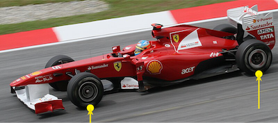
Fig. 5.1 Fernando Alonso racing on the circuit in Malaysia[3].#
5.5. Kinetic energy of rotation#
Naturally, a rotating object has kinetic energy - its parts are moving after all (even if they’re just rotating around a fixed axis). The total kinetic energy of rotation is simply the sum of the kinetic energies of all rotating parts, just like the total translational kinetic energy was the sum of the individual kinetic energies of the constituent particles in Section 4.5. Using that \(v = \omega r\), we can write for a discrete collection of particles:
by the (5.13) of the moment of inertia \(I\). Analogously we find for a continuous object, using (5.14):
so we arrive at the general rule:
Naturally, the work-energy theorem (eq. (3.8)) still holds, so we can use it to calculate the work necessary to effect a change in rotational velocity, which by equation (5.12) can also be expressed in terms of the torque (in 2D):
5.6. Angular momentum#
In analogy with the definition of torque, \(\bm{\tau} = \bm{r} \times \bm{F}\) as the rotational counterpart of the force, we define the angular momentum \(\bm{L}\) as the rotational counterpart of momentum:
For a rigid body rotating around an axis of symmetry, the angular momentum is given by
where \(I\) is the moment of inertia of the body with respect to the symmetry axis around which it rotates. Equation (5.24) also holds for a collection of particles rotating about a symmetry axis through their center of mass, as readily follows from (5.13) and (5.23). However, it does not hold in general, as in general, \(\bm{L}\) does not have to be parallel to \(\bm{\omega}\). For the general case, we need to consider a moment of inertia tensor \(\bm{I}\) (represented as a \(3 \times 3\) matrix) and write \(\bm{L} = \bm{I} \cdot \bm{\omega}\). We’ll consider this case in more detail in Section 7.3.
5.7. Conservation of angular momentum#
Given that the torque is the rotational analog of the force, and the angular momentum is that of the linear momentum, it will not come as a surprise that Newton’s second law of motion has a rotational counterpart that relates the net torque to the time derivative of the angular momentum. To see that this is true, we simply calculate that time derivative:
because \(\dot{\bm{r}} \times \bm{p} = \bm{v} \times m\bm{v} = 0\). Some texts even use equation (5.25) as the definition of torque and work from there. Note that in the case that there is no external torque, we arrive at another conservation law:
Theorem 5.3 (Law of conservation of angular momentum)
When no external torques act on a rotating object, its angular momentum is conserved.
Conservation of angular momentum is why a rolling hoop keeps rolling, and why a balancing a bicycle is relatively easy once you go fast enough.
What about collections of particles? Here things are a little more subtle. Writing \(\bm{L} = \sum_i \bm{L}_i\) and again taking the derivative, we arrive at
Now the sum on the right hand side of (5.26) includes both external torques exerted on the system, and internal torques exerted by the particles on each other. When we discussed conservation of linear momentum, the internal momenta all canceled pairwise because of Newton’s third law of motion. For torques this is not necessarily true, and we need the additional condition that the internal forces between two particles act along the line connecting those particles - then the internal torques are zero, and equation (5.25) holds for the collection as well. Consequently, if the net external torque is zero, angular momentum is again conserved.

Fig. 5.2 Five types of billiard shots. (a-c) The type of motion depends on where the cue hits the ball. (a) If the cue hits the ball at exactly \(7R/5\) above the table, the ball will exhibit pure rolling motion, \(\omega = v / R\). (b) If the cue hits the ball above the critical spot, it will rotate faster than translate (\(\omega > v / R\)) and exhibit a slipping rotation. Friction will slow down the rotation and accelerate the translation until rolling motion is achieved. (c) If the cue hits the ball below the critical spot, it will translate faster than rotate (\(\omega < v / R\)) and initially slide, until friction both slows down the translational speed and accelerates the rotational speed to the point where rolling motion is achieved. Note that the rotational motion may even be retrograde, i.e., backwards compared to the translational motion. (d-e) Behavior of the incident billiard ball before and after collision with a stationary ball of equal mass. Since the collision is elastic, all linear momentum is transferred to the other ball. If the incident ball was initially rolling, immediately after the collision it will continue rotating with complete slipping. Friction then causes the ball to pick up linear speed again, with a direction depending on the direction of the rotational motion, resulting in a follow (d) or draw (e) shot.#
5.8. Rolling and slipping motion#
When you slide an object over a surface (say, a book over a table), it will typically slow down quickly, due to frictional forces. When you do the same with a round object, like a water bottle, it may initially slide a little (especially if you push it hard), but will quickly start to rotate. You can easily check that when rotating, the object loses much less kinetic energy to work than when sliding - take the same water bottle, either on its bottom (sliding only) or on its side (a little sliding plus rolling), push it with the same initial force, and let go: the rolling bottle gets much further. However, somewhat ironically, the bottle can only roll thanks to friction. To start rolling, it needs to change its angular momentum, which requires a torque, which is provided by the frictional force acting on the bottle.
When a bottle (or ball, or any round object) rolls, the instantaneous speed of the point touching the surface over which it rolls is zero. Consequently, its rotational speed \(\omega\) and the translational speed of its center of rotation \(v_\mathrm{r}\) (where the r subscript is to indicate rolling) are related by \(v_\mathrm{r} = \omega R\), with \(R\) the relevant radius of our object. If the object’s center of rotation moves faster than \(v_\mathrm{r}\), the rotation can’t ‘keep up’, and the object slides over the surface. We call this type of motion slipping. Due to friction, objects undergoing slipping motion typically quickly slow down to \(v_\mathrm{r}\), at which point they roll without slipping.
Suppose we started our object with a velocity \(v_0\). If there is no rotation, the only force changing its velocity is the constant frictional force \(F_\mathrm{friction} = \mu_\mathrm{k} F_\mathrm{N} = \mu_\mathrm{k} m g\), with \(m\) the mass of the object (equation (2.13)). The constant force results in a linear decrease in the translational speed (see Section 2.3): \(v(t) = v_0 - \mu_\mathrm{k} g t\). However, if our object can roll, there is a second contribution to the motion, due to the torque \(\tau_\mathrm{friction} = F_\mathrm{friction} R\) of the frictional force. Using the rotational analog of Newton’s second law, equation (5.12) (or writing \(L = I \omega\) and using equation (5.25)), we get an equation of motion for the rotational velocity:
Integrating equation (5.27) with initial condition \(\omega(t=0) = 0\) we get \(\omega(t) = \mu_\mathrm{k} m g R t / I\). While the object undergoes slipping motion, the translational speed thus linearly decreases with time, whereas the rotational speed linearly increases. To find the time and velocity at which the object enters a purely rolling motion, we simply equate \(v(t)\) with \(\omega(t) R\), which gives
Note that the time \(t_\mathrm{r}\) until fully rolling motion is achieved scales inversely with the friction coefficient, but the final rolling speed \(v_r\) is independent of the frictional force. The rolling speed does depend on the moment of inertia of your object - for a hollow cylinder it’s \(v_\mathrm{r} = \frac12 v_0\), whereas for a solid cylinder it’s \(v_\mathrm{r} = \frac23 v_0\). Once the object is rolling, its surface no longer moves with respect to the surface that it’s rolling on (as its instantaneous speed at the point of touching is zero). Consequently, the frictional force is much reduced, and the object can roll a large distance before it stops; in fact, the main force slowing it down once it is rolling is drag with the ambient air, which we could safely ignore when (kinetic) friction was still in the picture.
Example 5.1 (A cylinder rolling down a slope)
A massive cylinder with mass \(m\) and radius \(R\) rolls without slipping down a plane inclined at an angle \(\theta\). The coefficient of (static) friction between the cylinder and the plane is \(\mu\). Find the linear acceleration of the cylinder.

Fig. 5.3 Free body diagram of a cylinder rolling down a plane.#
Solution There are at least three ways to tackle this problem. For all three, it helps (as always) to make a sketch, indicating the relevant forces - see Fig. 5.3.
Method 1: Forces and torques. Let the friction force \(F_\mathrm{f}\) be positive in the direction up the plane. Then we have:
\[\begin{split}\begin{align*} F = ma \quad &\Rightarrow \quad mg \sin\theta - F_\mathrm{f} = m a \\ \tau = I \alpha \quad &\Rightarrow \quad F_\mathrm{f} R = \frac12 m R^2 \alpha \\ \text{no slipping} \quad &\Rightarrow \quad a = \alpha R. \end{align*}\end{split}\]The last two equations give \(F_\mathrm{f} = \frac12 m a\). Plugging this into the first equation gives
\[a = \frac{g \sin\theta}{1 + \frac12} = \frac23 g \sin \theta.\]Method 2: Energy. The total energy of the system is given by
\[E_\mathrm{tot} = K + V = \frac12 m v^2 + \frac12 I \omega^2 + m g h.\]If the cylinder rolls down the slope without slipping, its angular and linear velocities are related through \(v = \omega R\). Also, if it moves a distance \(\Delta x\), its height decreases by \( \Delta x \cdot \sin \theta\). Conservation of energy then gives:
\[\begin{split}\begin{align*} 0 &= \frac{\mathrm{d}E_\mathrm{tot}}{\mathrm{d}t} = \frac{\mathrm{d}}{\mathrm{d}t} \left[ \frac12 m v^2 + \frac12 I \left(\frac{v}{R} \right)^2 - m g x \sin\theta \right]\\ &= m v \dot{v} + I \frac{v \dot{v}}{R^2} - m g v \sin\theta \\ &= \left[ a + \frac12 a - g \sin \theta \right] m v, \end{align*}\end{split}\]where we used \(I = \frac12 m R^2\) for a massive cylinder in the last line. The linear acceleration \(a\) is thus given by \(a = \frac23 g \sin\theta\).
Method 3: Rotational version of Newton’s second law. At a given point in time, we can apply the rotational version of Newton’s second law to rotations about the point where the cylinder touches the surface (as the cylinder is rolling without slipping, this is the only motion at that point). Of the three forces in the system, two act at that point, so they have no lever arm. Only gravity has a nonzero lever arm of length \(R \sin \theta\), leading to a torque given by \(\tau_z = m g R \sin\theta\). By the rotational version of Newton’s second law, we have \(\tau = I \alpha\), where \(I\) is the moment of inertia about the pivot. Applying the parallel-axis theorem, we find \(I = I_\mathrm{cm} + m d^2 = \frac32 m R^2\) in this case, so we get an angular acceleration of
\[\alpha = \frac{\tau_z}{I} = \frac{m g R \sin\theta}{\frac32 m R^2} = \frac{2g}{3R} \sin \theta.\]The linear acceleration of the center of the cylinder due to the ‘rotation’ about this pivot is given by \(a = R \alpha = \frac23 g \sin\theta\).
5.9. Precession and nutation#
The action of a torque causes a change in angular momentum, as expressed by equation (5.25)). A special case arises when the torque is perpendicular to the angular momentum: in that case the change affects only the direction of the angular momentum vector, not its magnitude. Since the torque is given by the cross product of the arm and the force, this case arises when the angular momentum is parallel to either arm or force, or more generally, lies in the plane spanned by the force and arm. As a result, the angular momentum vector may start rotating about a fixed axis, a process known as precession. Due to the action of a second force (with associated torque), the angle between the angular momentum vector and the fixed axis (which we’ll call the \(z\)-axis) may also change, a process known as nutation.

Fig. 5.4 Precession of a spinning top. The top rotates about an axis which makes an angle \(\phi\) with the vertical (\(z\)) axis. The angular momentum of the top is parallel to the rotation vector. The arm between the pivot (where the top touches the supporting surface) and the center of mass is parallel to the angular momentum as well. Consequently, the torque of the gravitational force (which as always is pointed downward from the center of mass) is perpendicular to the angular momentum, and causes it to precess about the \(z\)-axis with a precession frequency \(\omega_\mathrm{p}\).#
The simplest example of a precessing system is that of a rotationally symmetric top, spinning about an axis that is not the vertical \(z\)-axis, see Fig. 5.4. In this case, the arm of gravitational force (pointing from the pivot at the origin to the center of mass of the top) is parallel to the angular momentum, which itself is parallel to the rotation vector, as \(\bm{L} = I \bm{\omega}\). The torque of gravity is thus perpendicular to the angular momentum. If we call the angle between \(\bm{L}\) and the \(z\)-axis \(\phi\), and work in cylindrical coordinates \((\rho, \theta, z)\), we can write \(\bm{L} = L_{xy} \bm{\hat{\rho}} + L_z \bm{\hat{z}}\), where \(L_{xy} = L \sin\phi\) is the projection of \(\bm{L}\) on the \(xy\)-plane, and \(\bm{\hat{\rho}}\) is the radial unit vector in the \(xy\)-plane (i.e., \(\bm{\hat{\rho}} = \cos\theta \bm{\hat{x}} + \sin\theta \bm{\hat{y}}\)). The gravitational torque is then given by:
where \(\bm{r}\) is the arm pointing from the origin to the center of mass, \(r\) its length, and \(\bm{\hat{\theta}}\) the angular unit vector in the \(xy\)-plane (i.e., \(\bm{\hat{\theta}} = -\sin\theta \bm{\hat{x}} + \cos\theta \bm{\hat{y}}\)). For the time derivative of \(\bm{L}\), we get:
where we used (see equation (15.4))
Equating (5.30) and (5.31), we find that \(\mathrm{d}L_{xy} / \mathrm{d}t = \mathrm{d}L_z / \mathrm{d}t = 0\), and
Equation (5.32) gives us the frequency of the precession about the \(z\)-axis. The associated precession rotation vector is given by \(\bm{\omega}_\mathrm{p} = \omega_\mathrm{p} \bm{\hat{z}}\).
Where precession, in terms of the angles used in this section, represents a change in \(\theta\), nutation is associated with a change in the tilt angle \(\phi\). It comes about in several cases, most commonly due to the action of a second force, and often results in a periodic motion (hence the name nutation, ‘nodding’). One example is the change in the Earth’s axis. As the axis is not perpendicular to the plane of Earth’s orbit (it presently makes an angle of about \(23.4^\circ\)), gravity from the sun exerts a net torque on the Earth’s rotation axis, causing it to precess with a period of about 25000 years. Consequently, the current polar star will only remain the polar star for a couple of centuries. Due to the torques exerted by the moon and the other planets, the Earth’s axis also nutates - with amplitudes from arcseconds to a few degrees, and periods that range widely, from 18.6 years due to the gravitational pull of the moon up to millennia due to other effects.
5.10. Problems#
Exercise 5.1 (Hand-powered drills)
Fig. 5.5 shows two hand powered drills.
With which of the two drills shown in Fig. 5.5 will you be able to exert a greater torque on the drill bit?
With which of the two drills shown in Fig. 5.5 will you be able to exert a greater rotational speed?
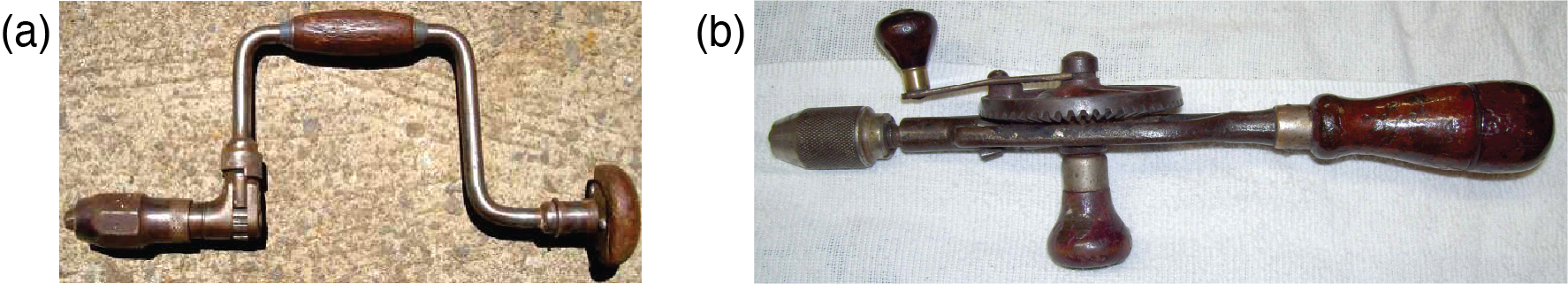
Fig. 5.5 Two hand-powered drills. (a) A brace [4], CC BY-SA 3.0. (b) An egg-beater drill [5].#
Exercise 5.2 (Atwood’s machine)
An Atwood’s machine consists of two masses \(m_1\) and \(m_2\), connected by a string that passes over a pulley. If the pulley is a disk of radius \(R\) and mass \(M\), find the acceleration of the masses.
Exercise 5.3 (Holding a pen)
You hold a uniform pen with a mass of \(25.0\;\mathrm{g}\) horizontal with your thumb pushing down on one end and your index finger pushing upward \(2.0\;\mathrm{cm}\) from your thumb. The pen is \(14\;\mathrm{cm}\) long.
Which of your fingers exerts the greater force?
Find the two forces.
Exercise 5.4 (Moment of inertia of a wagon wheel)
A wagon wheel is constructed as shown in the figure below. The radius of the wheel is \(R\). Each of the spokes that lie along the diameter has a mass \(m\), and the rim has mass \(M\) (you may assume the thickness of the rim and spokes are negligible compared to the radius \(R\)).

What is the moment of inertia of the wheel about an axis through the center, perpendicular to the plane of the wheel (figure a)?
For the same wheel, what is the moment of inertia for an axis through the center and two of the spokes, in the plane of the wheel (figure b)?
Exercise 5.5 (A sphere with non-uniform density)
A sphere with radius \(R = 0.200\;\mathrm{m}\) has a density \(\rho\) that decreases with distance \(r\) from the center of the sphere, according to \(\rho(r) = a - b r\), where \(a = 1.00\cdot 10^3\;\mathrm{kg}/\mathrm{m}^3\) and \(b = 4.00 \cdot 10^3\;\mathrm{kg}/\mathrm{m}^4\).
Calculate the total mass of the sphere.
Calculate the moment of inertia of the sphere for an axis through its center.
Exercise 5.6 (Yo-yo)
A \(0.10\;\mathrm{kg}\) yo-yo has an outer radius \(R\) that is \(5.0\) times greater than the radius \(r\) of its axle. The yo-yo is in equilibrium if a mass \(m\) is suspended from its outer edge, as shown in Fig. 5.6. Find the tensions \(T_1\) and \(T_2\) in the two strings, and the mass \(m\).

Fig. 5.6 A yo-yo with a mass suspended from its outer edge.#
Exercise 5.7 (Tipping a table)
A table consists of three pieces: a tabletop which is a circular disk of radius \(R\), thickness \(d = R/50\), and mass \(M\); a single leg that supports the tabletop in its center and consists of a hollow cylinder of height \(h=R/2\) and mass \(m = M/5\), and a foot, which consists of a solid cylinder of radius \(R/3\), mass \(M\) and height \(h=R/4\).
Find the position of the center of mass of this table.
With what force should you push down on the edge of the table to make it tip over?
A stone of mass \(m=M/2\) is placed on the table. How far out from the center can it be positioned before the table tips over? You may approximate the stone as a point mass.
Exercise 5.8 (A set-square protractor)
A set-square protractor made of plastic with density \(\rho = 1.2\;\mathrm{g}/\mathrm{cm}^3\), thickness \(2.0\;\mathrm{mm}\) and sides of \(10\;\mathrm{cm}\) is placed in a coordinate system as shown in the figure. The \(z\)-axis (not shown) is coming out of the paper.

Find the position of the center of mass of the protractor.
Find the moment of inertia of the protractor when rotating it along the y-axis.
Find the moment of inertia of the protractor when rotating it along the z-axis (i.e., the axis through the origin and perpendicular to the xy-plane).
Find the moment of inertia of the protractor when rotating it along an axis through its center of mass, and parallel to the z-axis (i.e., perpendicular to the xy-plane).
You pick up the protractor and balance it on your finger in its center of mass. You then tap one of the points with a small force F, directed in the plane of the protractor. For which of the three forces shown in figure b is the rotational speed the protractor gets the largest? (As always, explain your answer; the magnitude of all three forces is the same, the three indicated angles are all \(45^\circ\)).
You bring in three friends, who now push on the protractor along the directions indicated by \(F_1\), \(F_2\) and \(F_3\) in the figure. If \(F_1\) and \(F_2\) are both \(1.0\;\mathrm{N}\), how large must \(F_3\) be so that the protractor does not move?
Exercise 5.9 (A frame with four balls)
In this problem, we consider an object which consists of a frame with four balls, as depicted in the figure below. Each of the balls has a radius \(R = 5.0\;\mathrm{cm}\). Their masses are \(m_A = 3.0\;\mathrm{kg}\), \(m_B = 3.0\;\mathrm{kg}\), \(m_C = 2.0\;\mathrm{kg}\) and \(m_D = 1.0\;\mathrm{kg}\). The rods of the frame (which run from the edge of one ball to the edge of the next) have lengths \(L_1 = 20\;\mathrm{cm}\) and \(L_2 = 30\;\mathrm{cm}\) and a linear density \(\lambda = 10\;\mathrm{g/cm}\). (The distance between the centers of balls A and B is thus 30 cm, and between the centers of balls B and C is 40 cm). The thickness of the rods is negligible. We use the \(xyz\) frame indicated in the figure, with a \(z\) axis coming out of the paper in the origin.

Find the position of the center of mass of the object.
Find the moment of inertia of the object with respect to rotations about the \(y\)-axis.
We apply a torque of \(10\;\mathrm{Nm}\) to set the object spinning about the \(y\)-axis. Calculate the magnitude of the resulting angular acceleration.
Find the moment of inertia of the object with respect to rotations about an axis through its center of mass, and parallel to the \(y\)-axis.
Find the moment of inertia of the object with respect to rotations about an axis through its center of mass, and parallel to the \(z\)-axis.
Exercise 5.10 (A rotating triangle)
Three uniform bars with linear density (i.e., mass per unit length) \(\lambda\) are welded together into the shape of an isosceles triangle with sides of length \(5L\), \(5L\), and \(6L\) (figure a).

The moment of inertia of a rod with mass \(m\) and length \(L\) about an axis that goes through one of its end points at an angle \(\theta\) with the rod itself (figure b) is given by
Find the position of the center of mass of the triangle.
Find the moment of inertia of the triangle about its axis of symmetry. To do so, you may use the given expression for the moment of inertia of a bar at an angle.
Find the moment of inertia of the triangle about its longest side.
Find the moment of inertia of the triangle about the axis through its center of mass, perpendicular to the triangle’s plane. Use the theorems proved in this section to do so.
Are rotations of this triangle about its symmetry axis stable?
(Challenging) Derive the given expression for the moment of inertia of the rod under an angle.
Exercise 5.11 (Rolling cylinder)
We consider the same setting as in the worked example in Section 5.8. A massive cylinder with mass \(m\) and radius \(R\) rolls without slipping down a plane inclined at an angle \(\theta\) (see figure a). The coefficient of (static) friction between the cylinder and the plane is \(\mu\).

Find the largest angle \(\theta\) for which the cylinder doesn’t slip.
Suppose now that we accelerate the plane upwards (along its direction) with acceleration \(a\), see figure b. For what value of \(a\) does the center of mass of the cylinder not move? (You may assume that the cylinder still isn’t slipping).
Exercise 5.12 (Rolling wheel)
We consider a wheel with mass \(m\) and radius \(R\) which rolls without slipping on a flat (problems a and b) and an inclined (problems c-i) plane.

Draw a free-body diagram of the wheel rolling on a horizontal surface (figure a). Also indicate the (linear) velocity vector \(\bm{v}\) of the wheel.
How much work is done by the friction force on the wheel? What effect does this work have on the linear and angular velocity of the wheel? We now consider the case that the wheel rolls up an inclined plane (angle \(\alpha\), see figure b) with initial velocity \(v_0\).
Again draw a free-body diagram of the wheel and indicate the linear velocity \(\bm{v}\).
Determine the equation of motion for both the linear and the rotational velocity of the wheel (i.e. apply Newton’s second law to the translational and rotational motion ot the wheel). For this problem, you can describe the wheel as a cylindrical ring (and thus ignore the mass of the spokes).
Solve the equations of motion from (d) to obtain the linear acceleration of the wheel.
From the equations of motion, determine the magnitude and the direction of the frictional force acting on the wheel.
Determine the total energy of the wheel.
Take the derivative of the total energy of problem (g) to again arrive at an equation of motion for the wheel.
Is the energy of the wheel rolling up the incline conserved? Does the frictional force do any work in this case?
Exercise 5.13 (Moment of inertia of a solid cone)
We consider a solid cone of uniform density \(\rho\), height \(h\) and base radius \(R\).

Fig. 5.7 Sketch of the cone. (a) Dimensions. (b) Tilt angle \(\theta\).#
Taking the origin to be at the center of the base, and the symmetry axis along the \(z\) (vertical) axis, show that the center of mass of the cone is located at \((0, 0, h/4)\). Hint: consider the cone as a stack of disks and pick your origin carefully.
Over what maximum angle can you tilt the cone such that it just doesn’t fall over?
Qualitatively sketch the potential energy landscape \(U(\theta)\) of the cone as a function of this tilt angle \(\theta\). Indicate the stationary points and their stability. Assume the cone is narrow, i.e., the radius of the base is less than a quarter of the height.
Going back to the upright position, show that the moment of inertia of the cone around its axis of symmetry is given by \(I = (3/10) M R^2\), where \(M\) is the total mass of the cone.
Consider a cone which is \(100\;\mathrm{cm}\) high, has a base radius of \(20\;\mathrm{cm}\), and a mass density of \(700\;\mathrm{kg}/\mathrm{m}^3\). If the cone is standing with its base on a perfectly slippery surface (no friction), and you want to set it spinning at 1 revolution per minute, starting from rest, how much work do you have to do?
Exercise 5.14 (Collision between a puck and a hockey stick)
A hockey stick of mass \(m_\mathrm{s}\), length \(L\), and moment of inertia (with respect to its center of mass) \(I_0\) is at rest on the ice (which we assume to be frictionless). A puck with mass \(m_\mathrm{p}\) hits the stick a distance \(D\) from the middle (i.e., center of mass) of the stick. Before the collision, the puck was moving with speed \(v_0\) in a direction perpendicular to the stick, as indicated in the figure. The collision is completely inelastic, and the puck remains attached to the stick after the collision.

Find the speed \(v_\mathrm{f}\) of the center of mass of the stick + puck combination after the collision, in terms of \(v_0\), \(m_\mathrm{p}\), \(m_\mathrm{s}\), and \(L\).
After the collision, the stick and puck will rotate about their combined center of mass, which lies a distance \(b\) from the center of mass of the stick. Find \(b\).
What is the angular momentum \(L_\mathrm{cm}\) of the system before the collision, with respect to the center of mass of the final system? Use your answer at (b) to eliminate the value of \(b\) from your answer.
What is the angular velocity \(\omega\) of the stick + puck combination after the collision? Your answer should be independent of the variable \(b\).
Are the kinetic energy, linear momentum, and angular momentum conserved in this collision?
Exercise 5.15 (Another collision between a puck and a hockey stick)
We consider the same situation as in Exercise 5.14, but now the collision is fully elastic. Find the velocity of the puck after the collision, as well as the translational and rotational velocity of the stick after the collision. Hint: You have to solve for three unknowns, so you need three equation - what are they?
Exercise 5.16 (Sisyphus)
In Greek mythology Sisyphus by life was the king of Ephyra (Corinth). After he died, he was punished for his self-aggrandizing craftiness and deceitfulness in Tartarus (Greek hell) by being forced to roll an immense boulder up a hill, only for it to roll down when it nears the top, repeating this action for all eternity. We take the original rock to have a radius of \(1.00\;\mathrm{m}\) and a mass of \(2000\;\mathrm{kg}\); the hill is \(1.00\;\mathrm{km}\) high and has a slope of \(30^\circ\).
Suppose Sisyphus somehow managed to replace this rock with one made of aerogel with a mass of only \(1.0\;\mathrm{kg}\), covered by a thin layer of rock, which also has a mass of \(1.0\;\mathrm{kg}\). To hide his deceit, he still walks uphill slowly, and kicks the rock when it ‘slips’ down again. What speed must Sisyphus give the fake rock such that it has the same speed at the bottom as the real rock would have? You may assume that both rocks roll all the way down without slipping.
Hades, being not amused with Sisyphus’ trickery in part (a), decides to repay him using his own measures. He sends Sisyphus off to Helheim (Norse hell), strapped to the original rock, which he kicks so hard that it reaches escape velocity (\(11.2\;\mathrm{km}/\mathrm{s}\)) while also spinning at a rate of \(190\) revolutions per second. How much energy did Hades put into the rock (you may ignore Sisyphus’ mass, he’s a ghost anyway)?
Hel, the ruler of Helheim, doesn’t want him either, so she picks up the capstone of a dolmen, with a mass ten times that of Sisyphus’ rock, and hurls it towards the oncoming Sisyphus. As it happens, Hel throws just hard enough that after the collision, Sisyphus (now stuck between the two rocks) is spinning in place. How fast did Hel throw her stone?
At what angular velocities do Sisyphus and his two rocks spin after the collision? To do the calculation, assume that the capstone has the same density as Sisyphus’ rock and has the shape of a cylinder with a radius of \(2.00\;\mathrm{m}\). Sisyphus is caught between the spherical rock and the flat end of the capstone; the rotation after the collision is about the new center of mass.
Dante finally finds a place for Sisyphus in Inferno (Christian hell). To get him there, he first removes the capstone, and then ties a \(100\;\mathrm{km}\) long rope to the rock, which at the other end is connected to Lucifer (down at the center of Inferno). Lucifer then hauls in the rope, with a speed of \(1.0\;\mathrm{m}/\mathrm{s}\). Unfortunately for Sisyphus, the removal of the capstone has resulted in him getting a small linear velocity of \(1.0\;\mathrm{cm}/\mathrm{s}\) in the direction perpendicular to the rope. When Lucifer has hauled in enough rope to put Sisyphus in the fourth circle of Inferno at about \(5\;\mathrm{km}\) from himself, what is the angular velocity of Sisyphus’ rock?
Exercise 5.17 (Merry-go-round)
Two children, with masses \(m_1 = 10\;\mathrm{kg}\) and \(m_2 = 10\;\mathrm{kg}\) sit on a simple merry-go-round that consists of a massive disk with a mass of \(100\;\mathrm{kg}\) and a radius of \(2.0\;\mathrm{m}\). The disk can rotate freely about its center, and is doing so at a frequency \(\omega_0\) of 5.0 revolutions per minute. A third child with mass \(m_3 = 10\;\mathrm{kg}\) runs towards the merry-go-round with a speed \(v_0\) of \(1.0\;\mathrm{m}/\mathrm{s}\), at an angle of \(30^\circ\) with the tangent to the merry-go-round’s edge (see figure). Once it reaches the merry-go-round, the child jumps on it, and continues rotating with the other two. Find the resulting rotational velocity of the merry-go-round with the three children.

Exercise 5.18 (Billiards)
When playing billiards, forces from the cue or from collisions act on the balls only for a short time. To analyze what happens, we’ll work with the impulse, the integral of the force over the time of the collision (see Section 4.4.3):
Analogously to the (linear) impulse, we can define an angular impulse by integrating over the applied torque
We choose our coordinate system such that the origin is at the center of the initial position of the billiard ball, the ball will move in the \(x\)-direction, and the axis around which the ball rotates is in the \(z\)-direction. The cue hits the ball at height \(h\) above the plane of the table, with the cue in the \(xy\) plane (so the ball is not deviating to the left or to the right; this is known as an English shot).
Argue that for an English shot, we have \(J_\mathrm{lin} = m \Delta v_x\) and \(J_\mathrm{ang} = I_z \Delta \omega_z\), where \(\Delta v_x\) is the change in the velocity of the center of mass and \(\Delta \omega_z\) the change in the angular velocity of the ball due to the cue hitting the ball.
Show that if the ball has radius \(a\) and the cue hits the ball at height \(h\) above the table, immediately after the shot the angular and linear velocity are related through
\[\omega_z = \frac52 \frac{h-a}{a^2} v_x.\]Prove that the ball will roll without slipping if and only if \(h = \frac75 a\). Hint: first find \(v_\mathrm{c}\), the speed of the ball at the point of contact with the table.
Prove the statement in the caption of Fig. 5.2(b), that for a high shot (\(h > \frac75 a\)), friction will cause an increase in the translational velocity of the center of mass of the ball.
Suppose that our ball has achieved pure rolling motion, and hits (head-on) another stationary billiard ball of equal size and mass. While in the collision all linear momentum is transferred to the other ball, as the balls exert no torque on each other, the first ball retains its angular momentum. Find the final linear and angular velocity of this ball after it is once again rolling. Hint: again start with \(v_\mathrm{c}\), the speed of the ball at the point of contact with the table, immediately after the collision.