10. Solids and fluids

10.1. Continuous materials

In part I, we considered almost exclusively collections of single particles or single objects. We studied their motion due to forces acting on them by such sources as springs, gravity, friction, and other particles, and we considered both linear and rotational motion. In this chapter we will do much of the same, but for continuous materials. Of course all materials are ultimately built out of molecules, but here we will consider length scales that are very large compared to those of the molecules. Consequently, the number of molecules in the material is so large that we can safely ignore their discrete nature. We have seen a little of this approach in Section 4.1 and Section 5.4, where we calculated the center of mass and moment of inertia of a continuous object. The fact that we now switch to continuous materials is not to say that the results of the previous chapters no longer hold. In fact, we will make use once more of Newton’s laws and the various conservation laws to derive new equations for our continuous materials in this chapter. First, however, we must make an important classification: there are two types of continuous materials, solids and fluids. The difference between them lies in their response to the application of forces, or rather pressures, on them.

10.2. Pressure

Forces act on a single point in space. That makes them ideal for describing situations with a limited number of particles, but somewhat impractical when we look at the continuous case when the number of particles gets very large. We therefore need a continuous analog of the force. Fortunately, you’re very familiar with one. Stick your finger in a bucket of water and it goes in easily, but push with your flat hand on the surface and it is much harder, even if you use exactly the same force. Likewise, if you push on a sharp surface with your finger this can be quite painful, but putting a piece of cardboard or cloth over it can make this quite easy. The reason is that for the continuous objects we’re talking about (the water in the first case, your finger in the second - it all comes down to relative scales), not only the force matters, but also the area over which it is applied. Spreading a force over a larger area reduces the pressure (the force on the sharp object is distributed over the cardboard), but increasing the area requires a larger force (your finger/hand entering the water). We define the pressure as the force per unit area:

(10.1)\[ p = \frac{F}{A}. \]

Pressure is a scalar quantity: the force in equation (10.1) is the component of the force normal (or perpendicular) to the surface \(A\) (and thus equal to the normal force acting on that surface). We can, however, write a vector version of equation (10.1) by assigning a vector to the surface itself: we define the vector \(\mathrm{d}\bm{A}\) to be the vector perpendicular to the small surface element \(\mathrm{d}A\), which allows us to write for the normal force \(\mathrm{d}\bm{F}_N\) acting on that piece of surface:

(10.2)\[ \mathrm{d}\bm{F}_N = p \,\mathrm{d}\bm{A}. \]

In a typical gas or liquid (which collectively we call fluids), the molecules move around at random. If the fluid is at rest, the motions all add up to zero. If we put the fluid in a container, however, there will be continuous collisions of the molecules with the walls of the container, resulting in forces acting on the walls. The total force, divided by the surface area of the container, is by definition the pressure in that piece of fluid.

Pressure is measured in newtons per square meter, or pascals: \(1\; \mathrm{Pa} = 1\; \mathrm{N} / \mathrm{m}^2\). Other units that are sometimes used are the bar (\(1\; \mathrm{bar} = 10^5\; \mathrm{Pa}\)), the atmosphere (\(1\; \mathrm{atm} = 1.01325 \cdot 10^5\; \mathrm{Pa}\)), and the pounds per square inch (\(1\; \mathrm{psi} = 6.8948 \cdot 10^3 \mathrm{Pa}\). The bar and atmosphere are close to the typical air pressure at sea level on Earth; the pounds per square inch unit stems from a set of units common in the USA. A common device to measure atmospheric pressure is the manometer, in which the ambient air displaces a column of (almost) incompressible liquid to compress a gas in a closed tube. Modern manometers often use water, but until recently manometers using mercury were common (which is quite a bad idea given how toxic mercury is). These devices have led to yet another unit for pressure, the millimeter mercury (\(1 \mathrm{mmHg} = 133.32 \mathrm{Pa}\)), or the number of millimeters the pressure of the air can move the mercury column in a standardized manometer.

10.3. Stress and strain

Pressure is the best known example of (physical) stress, which is the more general class of forces applied to extended objects. A few examples are shown in Fig. 10.1. Fig. 10.1a shows tensile stress, which occurs when you pull on the ends of a long object, like a rod. Like pressure, the tensile stress is the applied force per unit area, which for the rod consists of the two areas of the end surfaces. As a consequence of applying the force, the rod can deform: extend when you pull on it, compress when you push on it. For small forces, the rod will behave like a spring - the amount of deformation depends linearly on the applied force (or equivalently, applied stress), and when you remove the force, the object assumes its original shape. We call such deformations elastic. Larger forces cause the permanent deformation of the object; we call these plastic.

The amount of deformation is known as the strain of an object. The strain is a nondimensional quantity which is the ratio of the size of the deformation length to the total size of the (unstrained) object. For the tensile rod in Fig. 10.1a), the unstrained length is \(L\), and the application of the stress adds an amount \(\Delta L\). The strain in this case is given by simply \(\Delta L / L\). However, stresses don’t have to be applied along the long axis of an object, or even perpendicular to its surfaces. Fig. 10.1b shows a very different example. Here the object is sheared, which means that forces are applied parallel to its surface (you can imagine doing this with a hardcover book, for example). The shear stress is still the force per unit area, but the shear strain is defined as the amount of displacement in the direction of the force (\(\Delta x\)) divided by the height \(h\) of the object. Yet another example is the hydraulic stress of Fig. 10.1c, where the pressure of the ambient fluid exerts forces on every surface of the spherical object shown. Consequently, its volume, originally \(V\), has diminished by an amount \(\Delta V\) - so the strain is \(\Delta V / V\).

Fig. 10.1 Three types of deformation stresses. (a) Tensile stress. (b) Shear(ing) stress. (c) Hydraulic stress (or hydraulic pressure).

Stress is usually denoted by \(\sigma\). There are different conventions for the strain, including \(\varepsilon\), \(\gamma\) (which we’ll use) and \(u\). In all cases, a small stress leads to an elastic deformation, i.e., a strain which depends linearly on the stress, and a large stress to a plastic deformation. Fig. 10.2 illustrates this, showing the stress as a function of the strain. The graph has two special points: first the yield strength, the point where you go from elastic to plastic deformations, and second the ultimate strength, the point at which the material cannot deform any further and breaks.

Fig. 10.2 Stress as a function of strain for a typical object.

10.3.1. Elastic moduli

In the elastic deformation regime, the stress is linear in the strain, so there has to be a proportionality constant, which we call an (elastic) modulus: stress = modulus \(\times\) strain. Because the stress has the same dimension as a pressure, and the strain is dimensionless, the modulus also must have the dimensions of a pressure, and is measured in pascals. Different deformations come with different moduli. For tension/compression (Fig. 10.1a), we define the Young’s modulus \(E\):

(10.3)\[ \sigma = E \gamma = E \frac{\Delta L}{L}. \]

For shear deformations, we have the shear modulus, which is denoted by either \(\mu\) or \(G\):

(10.4)\[ \sigma = G \gamma = G \frac{\Delta x}{h}. \]

Finally, for hydraulic stress (where the stress is simply the pressure of Section 10.2, with a minus sign because the pressure is exerted along the inwards-pointing normal), we define the bulk modulus, denoted by \(K\) or \(B\):

(10.5)\[ \sigma = -p = K \gamma = K \frac{\Delta V}{V}. \]

Sometimes you’ll encounter not the bulk modulus but the compressibility of a material, which is simply its inverse.

10.3.2. Poisson ratio

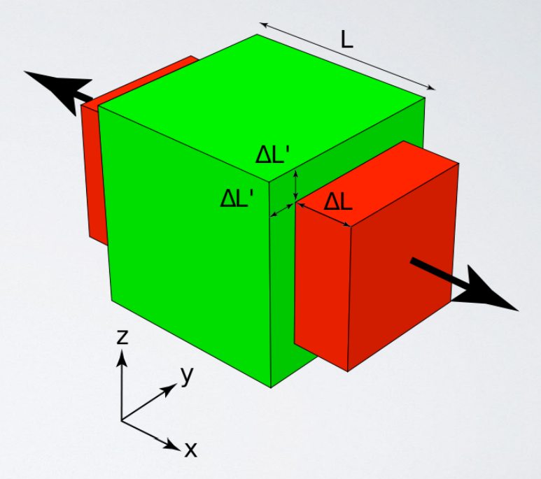
When you stretch a band of rubber (or any other elastic material), it doesn’t just get longer - it gets narrower as well. This feature of elastic solids is known as the Poisson effect, and characterized for different materials by their Poisson ratio. Roughly speaking, the Poisson ratio is the ratio between the change in the length in the transverse direction (perpendicular to the direction you’re pulling in) to that in the longitudinal or axial direction (the direction in which you’re pulling). More precisely, it is the ratio of the change in the strain in those directions. For pulling in the \(x\)-direction, we have (see also Fig. 10.3):

(10.6)\[ \nu = - \frac{\mathrm{d}\gamma_y}{\mathrm{d}\gamma_x} = \frac{\Delta x}{\Delta y}. \]

Note that the Poisson ratio \(\nu\) is a dimensionless quantity. For two-dimensional objects it can take values up to \(1\), for three-dimensional values its maximum is \(1/2\). Remarkably, it is possible to have a negative Poisson ratio: you can construct materials which expand when you pull on them.

Fig. 10.3 Possion effect: a tangential stress in one direction causes the object to extend in that direction, and compress in the directions perpendicular to it. The Poisson ratio \(\nu\) is defined as the ratio of the changes in the lengths in these directions (or more precisely, as the ratio of the changes in their strains), equation (10.6).

You might wonder if all the moduli we have introduced above are independent - if, for example, we know the bulk modulus and the Young’s modulus, can we derive the Poisson ratio or the shear modulus? The answer is yes - you need only two of these numbers to qualify any homogeneous elastic material, the others can then be calculated. To illustrate, the dimensionless Poisson ratio is given in terms of two of the three moduli defined above by:

(10.7)\[ \nu = \frac12 - \frac{E}{6B} = \frac{3B-2G}{2(3B+G)} = \frac{E}{2G} - 1. \]

From the various equalities in equation (10.7), relations between the various moduli (to calculate the third when the two others are given, or to calculate a modulus when one other and the Poisson ratio are given) can also be determined.

10.3.3. Bending

Apart from stretching, shearing and compressing them, solid objects like rods and plates can also be bent, deforming them from a straight to a curved shape. Bending is often significantly easier than stretching, as you surely know from practice: stretching a sheet of paper is virtually impossible, while you often have to make some effort to prevent even gravity from bending it. Likewise, a ruler or pointing stick can be bent by hand (though with considerable more effort than paper), but hardly compressed or stretched.

The reason why bending is so much easier than stretching or compressing is that bending involves no net change in volume. Bending is also easier than shearing, because when you bend something, you essentially apply a (very small) compression and extension on the inner and outer surface, respectively, which gives some internal shear, but much less than a global shear deformation. If your rod or plate (meaning any two-dimensional object) is thin enough, the amount of actual deformation involved is very small, and bending becomes easy. Even if you don’t ignore the thickness of the material, there is always a ‘neutral plane’ in the material when bending, for which there is no deformation at all.

The amount of work you need to do to bend a rod depends on two material properties: the Young’s modulus of the rod (because you’re compressing and extending away from the neutral plane) and the rod’s cross-sectional shape. The closer material is to the neutral plane, the less work you need to do to bend it. We can quantify this distribution of material with the second moment of the area \(I\), which is closely related to the moment of inertia we discussed in Section 5. If the rod is oriented along the \(z\)-axis, and we bend in the \(xz\)-plane, the second moment of the area is given by

(10.8)\[ I_y = \int x^2 \,\mathrm{d}A, \]

where the integral is over the cross-sectional area of the beam, and \(x\) the distance to the neutral plane. The subscript \(y\) indicates that we bend around the \(y\)-axis (giving a bent shape in the \(xz\)-plane). Table 10.1 lists the second moment of the area for some common shapes.

Table 10.1 Second moment of the area for some common cross-sectional shapes.

Shape	Second moment of the area
Massive cylinder, radius \(R\)	\(\frac{\pi}{4} R^4\)
Hollow cylinder, radius \(R\), thickness \(d\)	\(\pi R^3 d\)
Massive square, side \(a\)	\(\frac{1}{12} a^4\)

The effective flexural rigidity of a beam is given by the product of its Young’s modulus \(E\) and the second moment of the area \(I\). For a relatively thin beam, the neutral plane can be described by a function \(w(z)\), where \(z\) is the coordinate along the length of the beam. Under the assumption that the cross-section of the beam stays perpendicular to the neutral plane, the shape of the beam is given by the Euler-Bernoulli beam equation:

(10.9)\[ \frac{\mathrm{d}^2}{\mathrm{d}x^z} \left( E I \frac{\mathrm{d}^2 w}{\mathrm{d}z^2} \right) = q(z), \]

where \(q(z)\) is the load (force per unit length) applied to the beam. Often, the flexural rigidity is constant and can be pulled out of the derivative on the left. The load is often either a constant across the beam, or a collection of point forces, which can be written as Dirac delta functions. In both cases, finding the shape of the beam is a matter of integration.

The derivation of equation (10.9) is already nontrivial^[1]; for a plate, things become significantly more challenging. For small deflections, the governing equation is similar to the Euler-Bernoulli beam equation. The function \(w(x, y)\) now describes the deformation of the plate away from the flat configuration in the \(xy\)-plane; the corresponding equation is known as the Germain-Lagrange plate equation:

(10.10)\[ \nabla^2 \nabla^2 w = \frac{\partial^4 w}{\partial x^4} + 2 \frac{\partial^4 w}{\partial x^2 \partial y^2} + \frac{\partial^4 w}{\partial y^4} = \frac{q}{D}, \]

where \(q\) is again the load (now force per unit area) and the constant \(D\) is a combination of the plate’s Young’s modulus \(E\), Poisson ratio \(\nu\), and its thickness \(h\):

\[ D = \frac{2 h^3 E}{3 (1-\nu^2)}. \]

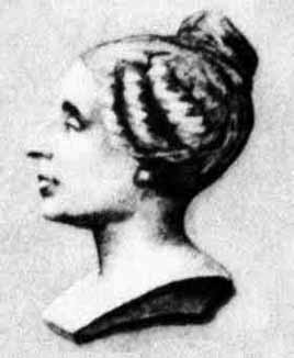
Sophie Germain (1776-1831)

Sophie Germain (1776-1831) was a French physicist and mathematician who lived during the revolutionary period in France and managed to study and contribute to science despite having little to no access to education. A teenager during the early revolutionary years, often unable to leave home due to the streets being unsafe, she studied mathematics using the books she found in her father’s library. When she was 18, the ‘{E}cole polytechnique opened, but as a woman she was not allowed to study there. However, the notes from the lectures given at the new school were made publicly available, allowing Germain to study them nonetheless. She quickly started corresponding with Lagrange, one of the founding faculty members, and later Legendre and Gauss as well. Germain made key contributions to finding the equations describing deformations of thin elastic plates, which she could do as submissions to a contest organized by the Paris academy of sciences. Although it took several attempts, Germain eventually won the prize, the first woman to do so. Next to her contributions in physics, Germain also worked in number theory, especially on the proof of Fermat’s last theorem. Despite support by Gauss, who advocated that she’d be given a honorary degree for her work, Germain never got a formal university degree. Things changed after her death, and various things have been named after her, including a prize awarded by the French Academy of Sciences.

Fig. 10.4 Portrait of Germain ^[2].

10.3.4. Buckling

Because bending a (thin) rod or plate requires much less work than compressing it, when compressing a plate or beam you quickly reach a point where the simple compressed deformation becomes unstable compared to a bent one. The transition from compressed to bent state is known as buckling. Exactly when a beam or plate buckles depends on the boundary conditions you apply; for example, if one end of a beam is free to move sideways, the buckling will result in a different shape, and therefore occur at a different compressional stress, than for the case when the beam is clamped at both ends. Although the phenomenon has been known for centuries, it became important only when large iron constructions like the Eiffel tower and various rail bridges were first built. Preventing buckling in construction is still a key point in engineering and architecture, and it remains an area of active research.

10.4. The response of solids and fluids to the application of stress

So far we’ve considered only solids, but in Section 10.1 we said we were going to look at the difference between solids and fluids. That difference lies in the response to an experiment in which you apply a stress to a sample of the material. As we’ve discussed in the previous two sections, applying a stress to a solid will cause it to deform. Now imagine what happens when you apply a stress to a liquid. Simply stick your hand in a bucket of water and move it, or put your flat hand on the surface and again move it. What will happen of course is that the water will start to flow. You are probably so familiar with these phenomena that this may seem almost tautological, but the response to stress is the fundamental difference between solid and fluid materials. To be more precise, it matters what happens with the energy. Deforming a material by applying a stress is performing work, so this requires you to put in some energy. However, once you release the stress, the deformation (as long as it was elastic) is reversed, and the energy returned, no matter how long you kept the stress in place. This is true for all kinds of stress, both transverse and shear. For fluids, however, the story is quite different. Applying a uniform hydraulic stress (a pressure on the outside of a container for example) will do the same to a fluid as to a solid (compress it, without flow). Applying a pressure to one side (thus creating a pressure difference) will create a flow, which for an ideal (frictionless) fluid is energy-conserving, but in a different fashion: the work you put in on the side of the increased pressure can be extracted on the other side from the flowing fluid. You can also cause a fluid to flow by applying a shear stress to it, in which case the flow is purely dissipative, which means that all the mechanical energy you put into it is dissipated (or ‘lost’) to friction and ultimately heat. An ideal fluid will not flow under shear stress, because the only way such a stress can be transferred is through friction. Moreover, for a non-ideal fluid, there will be dissipation in the first kind of flow as well.

Because solids deform due to the application of stresses, we typically want to calculate the amount of deformation - the strain \(\gamma\). Fluids flow, so what we want to find is the fluid velocity \(\bm{v}\) as a function of both position in space \(\bm{x}\) and time \(t\). The function \(\bm{v}(\bm{x}, t)\) is also sometimes referred to as the velocity field or flow field of the fluid, where the term ‘field’ refers to the fact that we don’t just want to know the velocity of a single particle, but of a continuous material that takes up a volume in space, and we want to find the velocity at each point in this volume. As we’ve seen above, fluid flows can be caused by pressure differences (or gradients) and by shearing, and can be conservative and dissipative - or of course a mixture of both. Similar to the moduli which relate stress and strain for solids, we can also characterize the amount of dissipation in non-ideal fluids by means of a number: the viscosity. The viscosity of a fluid is a measure of how strongly it resists stresses - higher viscosity means that the same stress will cause a lower flow velocity, as the rate of energy dissipation is higher. To measure viscosity, we can do a shear experiment, as illustrated in Fig. 10.5. We hold an amount of fluid between two solid plates a distance \(h\) apart. The bottom plate is fixed; we apply a horizontal force \(F\) to the top plate, or rather a stress \(\sigma = F/A\), causing it to move with a continuous speed \(v_\mathrm{top}\). Note that this happens only when the energy is completely dissipated - otherwise the top plate would accelerate. The fluid immediately next to the top plate gets dragged along with it: there is no slip, and their velocities are the same (this is known as the no-slip boundary condition, and holds for low speeds). Because the velocity of the bottom plate is zero, we end up with a velocity gradient \(\partial v / \partial z = v_\mathrm{top} / h\), and a height-dependent velocity field \(v(z) = (z/h)*v_\mathrm{top}\) towards in the positive \(x\) direction. If the top plate moves a distance \(\mathrm{d}x\) in a time interval \(\mathrm{d}t\), then the angle \(\theta\) as indicated in the figure is given by:

(10.11)\[ \tan \theta \approx \theta = \frac{\mathrm{d}x}{h} = \frac{v_\mathrm{top} \, \mathrm{d}t}{h}. \]

We can now define the strain rate \(\dot{\gamma}\) (the amount of deformation per unit time) by taking the limit \(\mathrm{d}t \to 0\):

(10.12)\[ \dot{\gamma} = \lim_{\mathrm{d}t \downarrow 0} \frac{\theta}{\mathrm{d}t} = \frac{v_\mathrm{top}}{h} = \frac{\partial v}{\partial z} = \frac{\sigma}{\eta}, \]

so

(10.13)\[ \sigma = \eta \dot{\gamma}, \]

and the viscosity \(\eta\) is the proportionality factor between the stress and the strain rate, like the different moduli were the proportionality factors between the stress and strain for elastic solids. Viscosity is also occasionally indicated as \(\mu\), has the dimensions of pressure times time, and is measured in \(\mathrm{Pa}\cdot\mathrm{s}\).

Fig. 10.5 Plate shear experiment. An amount of fluid is held between two solid plates. The bottom plate is fixed, the top plate moves to the right with a velocity \(v_\mathrm{top}\), resulting in a displacement \(\mathrm{d}x\) per time interval \(\mathrm{d}t\).

10.5. Non-Newtonian fluids and solid-fluid hybrids

Fluids for which the linear stress-shear rate relation (10.13) holds are known as Newtonian fluids. Some liquids you’ll encounter in daily life, such as water, olive oil, and shampoo, behave to good approximation as Newtonian. There are however also many fluids which behave differently, particularly in biological systems. Famous examples are quicksand, in which you sink deeper if you struggle, and maizena (corn starch), which when added to a pool, will allow you to walk on water if you do so fast enough, but if you sink in, pulling out will prove very difficult (there are of course numerous YouTube videos showing this). The reason for this odd behavior is that the shear rate and stress are not linearly related for these fluids. We distinguish two types of non-Newtonian fluids, see Fig. 10.6: shear-thinning ones, where the slope of the stress-strain rate line decreases with \(\dot{\gamma}\), and shear-thickening ones, where the slope increases with \(\dot{\gamma}\).

Going one step further, there are also materials that exhibit the properties of both fluids and solids, depending on the specific stresses and strains at hand. An example is mayonnaise, which is an emulsion of oil droplets in another fluid such as egg yolk or vinegar. Mayonnaise is a Bingham plastic, a material that behaves as a rigid body at low stress and as a viscous fluid at high stress, making it a viscoplastic material (see Fig. 10.6).

A final important class is that of viscoelastic materials. For these materials, which also exhibit properties of both viscous fluids and elastic solids, the stress-strain behavior depends on time. For example, if you apply a constant stress to them, they will not immediately flow (like a fluid would), but the stress will cause an increasing strain as time goes by, known as creep (the material is ‘crawling’). Inversely, if you impose a constant strain, this will initially correspond to a certain stress, as in a solid, but that stress will dissipate over time. Therefore, an experiment done on a viscoelastic material will trace out a look in a strain-stress diagram, which means it exhibits hysteresis: unloading releases less energy than was required for loading, resulting in dissipation in a loading-unloading cycle.

Fig. 10.6 Stress vs. strain rate for various kinds of fluids and a Bingham plastic, an intermediate between fluids and solids.

10.6. Stress and strain in multiple directions: stress and strain tensors*

There is a notable difference between the tensile strain (Fig. 10.1a) and the shear strain (Fig. 10.1b). For tensile strain, we take the ratio of the deformation and the object’s length in the same direction, while for shear strain, we take the ratio of the deformation to the object’s length in the perpendicular direction. Both are strains, but they represent different experiments - putting on a tensile and a shear stress, respectively. The two experiments can also be mixed: we could apply forces that are neither parallel nor perpendicular to any surface of our object. To deal with such a situation, we can decompose that force in parallel and perpendicular components, and try to take things from there. As long as the stress-strain relation is linear, we can then calculate the respective deformations and add them up to get the total deformation of the object. We can do this calculation fairly easily and definitely more quickly than by explicit decomposition by writing the stress and strain as two-tensors. A two-tensor is a linear map from one vector to another - which means that, given a basis, they can be written as matrices, and will act as such.

Note that a two-tensor is not the same as the matrix representing it, just like a vector (a one-tensor) is not the same as the string of numbers you associate it with. Instead, vectors and tensors are physical quantities, with a meaning independent of their representation. If you change coordinates, the numbers in the representations will change, but the physical properties (e.g. the length of the vector, or the trace of the two-tensor) will not. In practice, however, as long as you stay in the same basis, you can treat the two-tensor (which we’ll just call tensor) as equivalent to its matrix representation, just like we do with vectors.

The components of the strain tensor are defined as ratios of deformations to object lengths, like the tensile and shear strain. For a two-dimensional object, the two tensile and two shear strains make up all components, and we have:

(10.14)\[\begin{split} \bm{\gamma} = \left( \begin{array}{cc} \frac{\Delta x}{L_x} & \frac{\Delta x}{L_y} \\ \frac{\Delta y}{L_x} & \frac{\Delta y}{L_y} \end{array} \right). \end{split}\]

Although it captures all information, equation (10.14) is not very satisfying, for two reasons. First, it requires the use of specific deformations \(\Delta x\) and \(\Delta y\). If we want to calculate how much the object deforms under a given stress, this is not a convenient way of handling things, as we’d have to do calculations for each choice of deformation. Instead, we make use of the fact that \(\delta x / L_x\) is simply the derivative with respect to \(x\) of the function \(L_x(x,y)\). Second, the expression given in equation (10.14) is asymmetric in \(x\) and \(y\), which is not due to any physical reason, but to the fact that we chose a certain coordinate system. After all, for a uniform object, it should not matter in which direction you shear it, the shear strain should always be the same. Therefore we will symmetrize the expression, averaging over the two directions. This gives us a new expression for the strain tensor \(\bm{\gamma}\):

(10.15)\[\begin{split} \bm{\gamma} = \frac12 \left( \begin{array}{cc} 2\frac{\partial L_x}{\partial x} & \frac{\partial L_x}{\partial y} + \frac{\partial L_y}{\partial x} \\ \frac{\partial L_x}{\partial y} + \frac{\partial L_y}{\partial x} & 2\frac{\partial L_y}{\partial y} \end{array} \right). \end{split}\]

Analogous to the strain tensor, we also can consider the stress tensor, where each component represents the interaction between the direction of the force and the surface it acts on. An illustration in two and three dimensions is given in Fig. 10.7. By definition, the force on the surface with normal \(\bm{\hat{n}}\) is given by

(10.16)\[ \bm{F} = \bm{\sigma} \cdot \bm{\hat{n}} \]

Fig. 10.7 Components of the stress tensor and body force in (a) 2D and (b) 3D.

For a linear elastic material, the stress and strain are still related through elastic moduli. For example, for uniform compression, we have \(\gamma_{ij} = (\Delta V / V) \delta_{ij}\), where \(\delta_{ij}\) is the Kronecker delta, which is \(1\) for \(i=j\) and \(0\) for \(i \neq j\). The stress in that case is \(\sigma_{ij} = - p \delta_{ij}\), where \(p\) is the hydraulic pressure in the sample. The relation between the stress and the strain is still the bulk modulus \(K\), so we recover equation (10.5). Likewise, for a shear deformation (say a deformation in the \(x\) direction with two plates separated in the \(y\) direction), we have \(\sigma_{xy} = G \gamma_{xy}\) and all other components of \(\sigma\) and \(\gamma\) vanish.

The general relation between the stress and strain tensors generalizes Hooke’s law. In terms of the bulk and shear modulus, it is given by

(10.17)\[ \sigma_{ij} = K \mathrm{Tr}(\gamma) \delta_{ij} + 2 G \left( \gamma_{ij} - \frac13 \mathrm{Tr}(\gamma) \delta_{ij}\right), \]

where \(\mathrm{Tr}(\gamma) = \sum_k \gamma_{kk}\) is the trace of \(\gamma_{ij}\) (i.e., the sum of its diagonal elements). Equation (10.17) holds in three dimensions; in two dimensions the fraction \(\frac13\) in the second term is replaced by \(\frac12\). Equation (10.17) can be rewritten in terms of the Young’s modulus and Poisson ratio, in which case we find

(10.18)\[ \sigma_{ij} = \frac{E}{1+\nu} \left(\gamma_{ij} + \frac{\nu}{1-2\nu} \mathrm{Tr}(\gamma) \delta_{ij}\right). \]

---

[1]

See e.g. chapter 2 of Soft matter.

[2]

Portrait of Sophie Germain. Picture is a faithful reproduction of a two-dimensional public domain work, retrieved from Wikimedia commons