
13. The basic principles of thermodynamics#
Thermodynamics is the study of heat, its connection to energy, and the static (equilibrium) and dynamic properties of systems that have a thermal component. In a similar fashion as mechanics is based on a few axioms (Newton’s laws of motion and the various force laws), thermodynamics is based on a number of laws which are taken as axioms. The zeroth law (so labeled because it was formulated after the first, but more fundamental) deals with the concept of thermodynamic equilibrium; the first law is an extension of the concept of conservation of energy, and the second law tells us about the natural direction of heat flow. We will discuss these laws and their consequences in detail in this chapter.
13.1. Equilibrium#
Thermodynamic equilibrium is a state in which several different sub-classes of equilibrium all have to be present. To illustrate them, we will imagine a container that is fully isolated from the outside world, and subdivided into two compartments (Fig. 13.1). The two compartments are in thermodynamic equilibrium with each other if they are in mechanical, thermal and chemical equilibrium.
The three types of equilibrium that together constitute thermodynamic equilibrium are illustrated in Fig. 13.1. We have encountered mechanical equilibrium before. A mechanical object is in equilibrium when both the sum of the forces and the torques acting on it are zero. Suppose the dividing wall between the two compartments of our container can move, but the outside walls are rigidly fixed. Then, if the air pressure in one (say the left) compartment is larger than in the other, there will be a net force on the wall, which will move it towards the right, reducing the right compartment’s volume, and expanding that of the left compartment. This goes on until the pressure in both compartments is the same - i.e., they both exert the same force (per unit area) on the wall, at which point there is mechanical equilibrium.
Now suppose that the wall separating the two compartments cannot move, but heat exchange is possible. Then, if the left compartment is warmer than the right one, heat will flow from the left to the right - a phenomenon you have undoubtedly experienced many times yourself when trying to hold a paper cup of hot coffee. Consequently, the temperature of the colder compartment will rise, whereas that of the hotter one will drop, until they are equal and have reached thermal equilibrium. In fact, temperature can be defined by this property: if two systems are in thermal equilibrium (i.e., there is no net heat flow), then they have the same temperature.
Finally, suppose that particles can be freely exchanged between the two compartments. Clearly if all particles are in one compartment, there is an imbalance that will not be stable, as some particles will move over to the other compartment over time, resulting in a net particle flow. Again, this goes on until the flow of particles from left to right balances that from right to left. The equivalent quantity to pressure and temperature for this type of exchange is called the chemical potential, and when there is no more net particle flow between the two compartments, they are said to be in chemical equilibrium.

Fig. 13.1 Illustration of thermodynamic equilibrium: exchange of heat equilibrates temperature, exchange of volume equilibrates pressure, and exchange of particles equilibrates the chemical potential. Note that energy, heat, volume and number of particles scale with the system size (we call them extensive variables), while temperature, pressure and chemical potential (the intensive variables) do not. The equilibrium conditions thus all involve intensive variables, and systems of different size can be in thermodynamic equilibrium with each other.#
13.1.1. The zeroth law of thermodynamics#
Suppose we have three systems, as in Fig. 13.2, where system 1 is coupled to system 2, and system 2 to system 3, but there is no direct coupling between systems 1 and 3. Then if there is thermodynamic equilibrium between systems 1 and 2, they have the same temperature, pressure and chemical potential. The same holds for systems 2 and 3. But then we have \(T_1 = T_2 = T_3\) (and the same for \(p\) and \(\mu\)), so systems 1 and 3 must also be in equilibrium, which gives us our first axiom of thermodynamics:
Axiom 13.1 (Zeroth law of thermodynamics)
If two systems are both in equilibrium with a third system, they are in equilibrium with each other.

Fig. 13.2 Illustration of the zeroth law of thermodynamics: when two systems are both in equilibrium with a third, they are in equilibrium with each other.#
13.2. Heat and energy#
In the example of the previous section, when there is no mechanical equilibrium, it can be reached by doing work, in this case moving the wall. This work originates from the pressure (a force per unit area) acting on the wall, resulting in a change of volume. It is therefore precisely the same kind of work we defined in Section 3:
In equation (13.1), \(\mathrm{d}r\) is the distance over with the wall moves, \(A\) the area of the (moving part of the) wall, and \(\mathrm{d}V = A \mathrm{d}r\) is the amount of volume added to the compartment with the larger pressure. The net force on the wall equals the difference in pressure, \(\Delta p = p_1 - p_2\) times the wall area; the difference in pressure (or net pressure) is usually just denoted \(p\) in thermodynamics. Equation (13.1) tells us that a pressure difference can be used to move objects, and thus that work can be extracted. However, if we are interested in the properties of the gas (that is, after all, the system which we are studying here), we should instead calculate the work done on the gas, which is minus the work done by the gas on the wall:
Equation (13.2) tells us that when the two compartments move towards mechanical equilibrium, mechanical energy is exchanged between them, until their pressures are equal. Similarly, we’ve defined thermal equilibrium as the state in which the temperatures of the two compartments are equal, and noted that an imbalance in temperature leads to a flow of heat. The key realization that lays at the foundation of thermodynamics is that this heat is also a form of energy. Microscopically, we can identify temperature as the kinetic energy of the constituent particles of a material, so an exchange in temperature between two systems, i.e. a heat flow, is simply an exchange in kinetic energy. With that in mind, the fact that heat is a form of energy is not so surprising. The great feat of the early explorers of thermodynamics was to realize this without having microscopic knowledge of the materials[1].
13.2.1. The first law of thermodynamics#
We will denote a transfer of heat (a heat flow between two systems of unequal temperature) by \(Q\). A transfer of energy in the form of mechanical work is still denoted by \(W\); the total transfer of energy between two systems can then be written as:
where \(\Delta U\) (sometimes also denoted \(\Delta E\)) is the change in internal energy of a system[2]. Equation (13.3) is the mathematical expression of our second axiom:
Axiom 13.2 (First law of thermodynamics)
The total change in internal energy of a system equals the sum of the net heat transfer to the system and the net work done on the system.
A direct consequence of this law is that, for an isolated system, the total internal energy is conserved. This statement is closely related to the conservation of the total energy of an isolated mechanical system (see Section 3.4). Note however that where in classical mechanics conservation of energy follows from Newton’s laws of motion, here we take its extended version (i.e., including heat) as an axiom for our theory.
Quite often, we will want to consider processes in which the heat exchange or work done changes during the process. For those, as we did above when defining the work as the integral over the (varying) force, we need to integrate over the process to find the total change in heat, work or energy. To do so, we use the differential form of the first law:
We already know that \(\mathrm{d}W = - p \mathrm{d}V\), which is simply the infinitesimal version of (13.2). As we’ll see in Section 14.3, we will find a similar expression for \(\mathrm{d}Q\), in terms of the temperature and a quantity called entropy[3]. Before that, however, we will take a macroscopic look at the heat flow \(Q\), starting with the second law.
13.2.2. The second law of thermodynamics#
In its simplest form, our third axiom states an observational fact that will probably not surprise you:
Axiom 13.3 (Second law of thermodynamics)
Heat cannot spontaneously flow from a cold to a hot reservoir.
Stated like this, the second law appears almost tautological - but don’t be fooled by simplicity: the consequences are quite profound, as we’ll see later. For now, we simply note two things. First, the second law is different from the first, in that the first tells you something about the total energy, i.e. the heat plus work, whereas the second tells you something about the flow of heat alone. Second, you might have noticed that the second law is very similar to another commonly known observational fact: water always flows downhill. The flow of water can of course be described by mechanics (and caused by the force of gravity); in close analogy, the flow of heat is described by thermodynamics and caused by a difference in temperature. Moreover, we may say that the flow of water represents a difference in potential energy between a high and a low point, which is well-defined exactly because water will never spontaneously flow uphill. Similarly, we will define a ‘thermodynamic potential energy’ later based on the flow of heat. This thermodynamic equivalent of the potential energy will be the entropy, as we’ll see in Section 14.3.
13.3. Macroscopic properties of heat#
13.3.1. Units of temperature#
By including heat in the axioms of thermodynamics, we’ve extended the repertoire of quantities we can measure. In mechanics, we could construct all quantities from three basic ones: length, time, and mass. To measure heat at a macroscopic level, we need a fourth quantity: temperature. Temperature is is measured in Kelvins (\(\mathrm{K}\)). The Kelvin scale is defined such that at \(T=0\;\mathrm{K}\) all atoms have kinetic energy 0 (‘absolute zero’), and a step of \(1\;\mathrm{K}\) corresponds to a step of \(1^\circ\mathrm{C}\). As you probably know, the common[4] Celsius scale has \(0^\circ\mathrm{C}\) as the freezing point of pure water and \(100^\circ\mathrm{C}\) its boiling point. Converting from one into the other, we find that water freezes at \(273.15\;\mathrm{K}\), so to get a temperature in Kelvin when you have one in degrees Celsius, simply subtract \(273.15\).
As we’ll see in Section 13.5, microscopically we can interpret the temperature of a material as the total kinetic energy of its constituent molecules, so there is a conversion factor between energy and temperature. This conversion factor is known as Boltzmann’s constant, and is approximately given by \(\kB = 1.38 \cdot 10^{-23}\;\mathrm{J}/\mathrm{K}\). Since the number of particles in a typical microscopic volume is very large, and \(\kB\) very small, it is practical to define a reference that is somewhat less unwieldy. To that end, we define Avogadro’s number \(N_\mathrm{A} = 6.022 \cdot 10^{23}\), which is the number of carbon-12 atoms in a sample of 12 grams. By definition, a mole of material (unit: mol) contains \(N_\mathrm{A}\) atoms of that material. The product of Avogadro’s number and Boltzmann’s constant is the amount of energy in a mole of (ideal) gas; it’s value is known as the ideal gas constant \(R = N_\mathrm{A} \cdot \kB = 8.314\;\mathrm{J}/\mathrm{K}\).
13.3.2. Heat capacity#
Unsurprisingly, the larger the difference in temperature between two bodies in thermal contact, the larger the heat flow between them. Probably also unsurprisingly, the relation turns out to be linear: to raise the temperature of a given body by twice as many degrees, you need twice the amount of energy. The proportionality factor is known as the heat capacity of the body (denoted \(C\)), and we can write:
If our body consists of a single substance, then its heat capacity scales with its mass. We can then define a (mass) specific heat of the substance (denoted \(c\), or, e.g., \(c_\mathrm{w}\) for water), which is simply its heat capacity per unit mass. In terms of mass and specific heat, we have
Water is a remarkable substance in many aspects (we’ll encounter more of them below), one being its high specific heat - \(c_\mathrm{w} = 4.184\;\mathrm{J}/\mathrm{kg}\cdot\mathrm{K}\), much higher than typical solids, which is why the sea warms up and cools down much more slowly than land, causing the difference in climate between coastal and inland regions.
Although the heat capacity \(C\) is a proportionality constant in equation (13.5), its value depends not only on the material in question, but also on the process, where we have multiple choices. Since the total internal energy of a thermodynamic system is the sum of the heat and the work, for measuring \(C\), it matters how we control the sample. The work is the product of a pair of conjugate variables: the pressure and the volume. We can experimentally control one of these at a time, but not both - so we could keep either the pressure or the volume constant, while measuring how the heat changes as a function of a change in temperature. Consequently, we get two different ways of determining the heat capacity, which in general results in two different values: the heat capacity at fixed volume, \(C_V\), and the heat capacity at fixed pressure, \(C_p\):
where the subscript indicates which parameter is held fixed.
13.3.3. Heat transfer#
Heat can commonly be transferred in three different ways. Like electricity, heat can be conducted well in some materials (e.g. metals), whereas others are good insulators (e.g. styrofoam). It can also be released from a hot body in the form of radiation. And it can be transported by a fluid by means of convection.
Conduction of heat happens when two objects, or two parts of the same object, are in direct physical contact. If one part has higher temperature than the other, heat will flow from the hotter to the colder part. This process is described by the heat equation:
Equation (13.8) describes the change of the heat function \(u\) (essentially the temperature) over time and space, governed by the thermal diffusivity \(\alpha\). It is mathematically equivalent to the diffusion equation which describes the spread over time of a chemical concentration.
For the heat flow through a uniform rod with cross-sectional area \(A\), the rate of the flow of heat per unit area, \(\bm{q}\), equals minus the temperature gradient across the rod:
where the material constant \(k\) is the thermal conductivity of the material. Equation (13.9) is known as Fourier’s law. The heat equation can be derived from Fourier’s law and conservation of energy. The latter gives that the rate of change of the internal heat in a small volume element in the material, \(\partial Q / \partial t\), must be equal to the flow of heat out of that volume element:
On the other hand, by definition of the temperature, the rate of change of heat is proportional to the rate of change of the temperature, \(\partial u/\partial t\):
where \(c\) is the specific heat and \(\rho\) the density of the material. Combining equations (13.9)-(13.11)), we retrieve the heat equation (13.8), with a relation between the thermal diffusivity and the thermal conductivity, \(\alpha = k / c \rho\).
For the specific case of steady-state heat flow through an object of thickness \(\Delta x\) and cross-sectional area \(A\), due to a temperature difference \(\Delta T\), we can write:

Fig. 13.3 Heat transport through convection. (a) Rayleigh-Bernard cells in a fluid that is heated from below. As the fluid heats up, it gets less dense and rises. At the top the fluid cools down, gets denser, and flows down again [5]. (b) Top view of convection cells on the surface of the sun, imaged by the Inouye Solar Telescope; the cell-like structures are about the size of Texas. Image credit NSO/NSF/AURA [6]; see also the video on the NSO website. (c) Illustration of convection cells in Earth’s atmosphere, resulting (in combination with Earth’s rotation and the Coriolis effect) in westerly and easterly currents [7].#
Convection of heat happens due to the fact that fluids have the property that their density decreases with temperature. Suppose now that we have a closed container filled with a fluid initially at a uniform temperature. At some point we start heating the container from below, raising the temperature of the fluid at the bottom. Because this decreases the fluid’s density, the hotter fluid will rise, and the colder fluid above will fall down, creating an instability which results in the formation of convective cells. This setup is known as the Rayleigh-Bernard cell, and convective cells are seen at many scales, from tabletop setups to planetary and solar atmospheric motion, see Fig. 13.3.
One obvious question to ask is when we get conduction and when we get convection in a fluid with a temperature gradient. These two methods of heat transfer somewhat resemble laminar and turbulent flow in fluid dynamics, where we typically get laminar flows at low values of the Reynolds number and turbulent flows at high values. For the transition from conduction to convection we have a similar number, the Rayleigh number \(\mathrm{Ra}\). The Rayleigh number measures the ratio of the time scales of motion due to conduction and convection. Suppose we have a box with sides \(L\) in which fluid has a density difference \(\Delta \rho\) between top and bottom, and consequently moves with speed \(v\). The force of gravity due to the density difference can be estimated as \((\Delta \rho) g L^3\), while the (Stokes) drag force on the moving fluid is approximately \(\eta L v\), with \(\eta\) the viscosity. Equating the two forces in a steady-state convective flow, we get \(v \sim (\Delta \rho) g L^2 / \eta\), or a typical timescale of \(L/u \sim \eta / (\Delta \rho) L g\). For the diffusive conductive flow, we can estimate the typical timescale as \(L^2/\alpha\). For the Rayleigh number, we then obtain
In the last equality of (13.13), we approximated \(\Delta \rho = \rho \beta \Delta T\), where \(\rho\) is the average density of the fluid, and \(\beta\) its thermal expansion coefficient, defined as[8]
The critical Rayleigh number (i.e., the value of \(\mathrm{Ra}\) at which we switch from conductive to convective heat flow) depends on the boundary conditions of the system. For a system with two free boundaries, the critical value was found by Rayleigh himself at approximately 657; for rigid boundaries at top and bottom, the critical value is almost three times higher at 1708.
The third form of heat transfer, radiation, occurs due to the emission of energy quanta, or photons, from an object that has larger temperature than its surroundings. These photons typically have wavelengths in the infrared, which is why you can measure the temperature of objects with infrared cameras. The radiative power of a hot object is given by the Stefan-Boltzmann law:
where \(T\) is the object’s temperature, \(A\) its area, \(\varepsilon\) its emissivity (ranging from 0 for a black hole to 1 for a perfect radiator, known as a black body), and \(\sigma = 5.67\cdot 10^{-8}\;\mathrm{W}/\mathrm{m}^2 \mathrm{K}^4\) the Stefan-Boltzmann constant. Note that for an object that does not sit in an environment which is at absolute zero temperature, there is also an influx of radiation given by equation (13.15), but now with \(T\) the temperature of the environment. The net radiation is the difference between the outgoing and incoming heat.
13.4. Phase diagrams#
As everyone knows from first-hand experience, water is present on our planet in three different kinds, or phases: solid (ice), liquid (usually just called water), and gas. We also often encounter the transitions between these, particularly as a function of temperature - liquid water can freeze to ice or boil ‘away’ into gas, ice melts, and gas condenses into water droplets. Ice can also directly turn to gas and vice versa (this is how snow disappears even when it’s not melting). Which phase water, or any other substance, happens to be in, depends on its state variables, such as temperature and pressure. A useful visualization of all this is given in a phase diagram. In its simplest form, when it describes a single substance as a function of just those two variables, we typically plot the temperature on the horizontal axis and the pressure on the vertical, and indicate regions in which the substance is in the solid, liquid or gaseous phase. Examples for some commonly encountered substances (such as nitrogen and carbon dioxide), and for the somewhat different case of water, are given in Fig. 13.4.
Unsurprisingly, at low temperatures and ‘ordinary’ (atmospheric, i.e., \(1\;\mathrm{atm} = 10^5\;\mathrm{Pa}\)) pressures, both water and carbon dioxide are solid, and when raising the temperature, they first melt and then boil, crossing first into the liquid and then the gaseous phase. Also, dependent on the temperature, gas at low pressure can by compression be forced to undergo a phase transition into the solid (low temperature) or liquid (higher temperature) phase. What might surprise you is that at high temperatures, the difference between gas and liquid disappears - there is no more phase transition above a certain critical temperature! The line separating the two phases ends in a critical point, and if you were to take a gas at low pressure, heat it up, then compress, and finally cool it down again, you could go from gas to liquid without encountering a phase transition. However, you would see one when you’d leave out the heating up and cooling down, and just compressed the gas. Therefore, the gas and liquid phase are both the same and different - they’re both fluids, but with different densities at low temperatures. Solids, on the other hand, are structurally different, and the line separating solids from liquids goes on indefinitely.
Next to the critical point, there is a second point of interest in the phase diagram: the triple point where the lines separating solid from liquid, solid from gas, and gas from liquid all meet. At this specific temperature and pressure all three phases can coexist, and a liquid there can boil and freeze at the same time.
Finally, note the difference between the more generic phase diagram, in which compressing a gas at moderately high temperatures induces a phase transition first to liquid, and then a second to a solid state. In contrast, for water, compressing the solid form (ice) can induce a phase transition into the liquid form (water)! This unusual property, together with the also unusual property that solid water has lower density than liquid water, makes ice skating possible. If the solid water were more dense than the liquid form (as is the case with virtually all other substances), it would sink, so you couldn’t stand on it (it wouldn’t even be at the surface). And because the ice melts (a little) when you exert pressure on it, exerting a high pressure with the blade of your skates produces enough liquid water to lubricate the skate, lowering the friction coefficient between blade and ice, and allowing you to move with ease. This only works down to a certain temperature though - as you can see in Fig. 13.4, lowering the temperature increases the amount of pressure you have to exert to melt the ice, so no skating under \(-20^\circ\mathrm{C}\) or so.

Fig. 13.4 Schematic phase diagrams of (a) a generic single-component substance (e.g. nitrogen, carbon dioxide) and (b) water.#
13.4.1. Heat of transformation#
Getting ice to melt or water to boil requires the addition of energy in the form of heat. Conversely, to get water to freeze you need to extract energy. The amount of energy per unit mass you need for these transformations is known as the heat of transformation
The various phase transitions have corresponding names for the heat of transformation; for example, for boiling a liquid we have the heat of vaporization \(L_\mathrm{v}\) and for melting a solid we have the heat of fusion \(L_\mathrm{f}\). For water, the corresponding values are \(L_\mathrm{f} = 334\;\mathrm{kJ}/\mathrm{kg}\) and \(L_\mathrm{v} = 2257\;\mathrm{kJ}/\mathrm{kg}\).
Example 13.1 (Mixing ice and water)
You add three ice cubes of \(15.0\;\mathrm{g}\) each, taken directly from a freezer at \(-18^\circ\mathrm{C}\), to a glass containing \(250\;\mathrm{g}\) of liquid water at room temperature (\(20^\circ\mathrm{C}\)). Will all the ice melt? If so, what is the resulting temperature of the mixture, and if not, how much ice is left?
Solution As the ice and the water are initially at different temperatures, heat will flow from the hotter (water) to the colder (ice) material until they are in thermal equilibrium. To heat the ice first to its melting point (\(0^\circ\mathrm{C}\)) will require an amount of heat given by (see equation (13.6), with numbers from Section 16.4):
Melting the ice would require an amount of energy given by (equation (13.16))
Cooling down the water to freezing point on the other hand would take an amount of heat equal to
As \(Q_1 + Q_2 < Q_3\), the ice will all melt. To find the resulting final temperature \(T_\mathrm{f}\) of the mixture, we equate the amount of heat coming from the water in the glass to the amount of heat added to the ice (which becomes water somewhere along the process):
Note that in this calculation, we exploited the fact that \(1^\circ\mathrm{C} = 1\;\mathrm{K}\). Also, we ignored the flow of heat from the glass to the environment - if you wait long enough, there will be thermal equilibrium between the water and the air in the room, so then the ice will definitely melt.
13.5. The kinetic theory of gases#
So far, we have treated our materials of interest as a continuum, which is to say that we’ve assumed (tacitly) that we could chop up our material into small parts, and those small parts would have the same properties as the larger amount we started with. For macroscopic systems, this assumption is justified, as illustrated by the fact that we have the staggering number of \(N_\mathrm{A} = 6.022 \cdot 10^{23}\) gas molecules in every mole of gas. We say that macroscopic systems can be described as being in the thermodynamic limit, which strictly speaking is a system in which we have taken the number of particles to infinity (and thus the particles themselves have to be infinitesimally small). However, we also know that all materials are built of small but finite-sized components - their molecules - so the continuum approximation should break down when we zoom in far enough. In this section we will make a start at connecting the microscopic world of the molecules to the macroscopic world of effectively continuous liquids and gases, a topic that will be studied in much more detail in statistical physics. Here we will exclusively focus on the ideal gas as a model system.
13.5.1. The ideal gas#
An ideal gas consists of point-like atoms that only interact with each other when they collide. Noble gases like helium, neon and argon are good approximations to this ideal. Ideal gases behave according to the ideal gas law, which relates the pressure \(p\), occupied volume \(V\) and temperature \(T\) of an ideal gas[9]:
In equation (13.17), \(N\) is the number of gas atoms, and \(\kB\) is Boltzmann’s constant, which, as we have seen in Section 13.3.1, converts a temperature into an energy. In the alternative form, \(n\) is the number of moles of gas, and \(R = N_\mathrm{A} \cdot \kB\) the ideal gas constant, with \(N_\mathrm{A}\) Avogadro’s number.
13.5.2. Temperature revisited#
In Section 13.3.1 we introduced temperature as a measure of the kinetic energy of the molecules in a substance (which we will take here to be a gas). For an ideal gas, the only energy is kinetic energy, because by definition, the molecules in an ideal gas do not exert any forces on each other, so they do not experience any potential, and their potential energy equals zero[10]. However, if we confine the gas by putting it in a container, the molecules can run into the walls of the container, and thus exert forces on those walls - and by bouncing off the walls, the walls exert forces on the molecules as well. Let us assume we have confined \(N\) molecules of an ideal gas in a container of dimensions \(L \times L \times L\). The molecules are free to move within the container, and we assume that this movement happens in random directions, and with a speed that is independent of the direction (we say that there is no ‘preferred direction’ for the molecules to move in). We also assume that any collisions the molecules have with the walls are fully elastic, so energy is conserved.
If molecule \(i\) crashes into one of the walls, it exerts a force \(\bm{F}_i\) on it, and by Newton’s third law, the wall exerts a reciprocal force \(-\bm{F}_i\) on the molecule. Let us pick coordinates such that the origin is at one of the corners of the box, and the walls are parallel to the various coordinate planes. Suppose particle \(i\) collides with the right-hand wall parallel to the \(yz\) plane, then obviously only its velocity component in the \(x\)-direction will change. More precisely, by conservation of momentum (since the wall will not move), the \(x\)-component will flip sign, and the particle will transfer a momentum \(2 m_i v_{xi}\) to the wall. The magnitude of the particle’s velocity in the \(x\)-direction will moreover not change, so we can calculate exactly how often it will collide with the right-hand wall: once every \(\Delta t_i = 2L/v_{xi}\) seconds. Therefore the rate of momentum transfer to the wall by this particle, which by Newton’s second law is simply the force exerted by the particle on the wall, equals \(F_i = \Delta p_i / \Delta t_i = m_i v_{xi}^2 / L\). The pressure is the force on the wall per unit area; if the number of molecules is large enough, we can average the forces they exert on each of the walls. Since the walls have an area of size \(A = L \times L\), we find that the walls all experience a pressure \(p\) given by:
In equation (13.18) we used that all particles in the gas have the same mass \(m\); in the last step we also introduced the average of the velocities squared \(\overline{v_x^2}\), and the container’s volume \(V = L^3\). Now picking the \(x\)-direction was of course completely arbitrary - we might just as well have picked the \(y\) or \(z\)-direction, and found the same result. In fact, as stated above, we assumed that the direction would not matter, or more precisely, that the magnitude of the velocity would be direction-independent. Therefore, we have \(\overline{v_x^2} = \overline{v_y^2} = \overline{v_z^2} = \frac13 \overline{v^2}\), where the last equality holds because the square of the magnitude of the velocity is simply the sum of the squares of its components. We can thus rewrite equation (13.18) in a direction-independent manner as
or
We recognize the expression in brackets on the right-hand side of equation (13.20) as the average kinetic energy of a particle in the gas, and the complete right-hand side therefore represents \(2/3\) of the total kinetic energy of the gas. On the left-hand side we find the combination \(pV\) that also occurs in the ideal gas law, which states that this quantity must equal \(N \kB T\); therefore we must have:
and we find that indeed temperature is a measure for the average kinetic energy of the particles in an ideal gas.
13.5.3. The Maxwell distribution#
In the previous section we related the (macroscopic) temperature of an ideal gas to the (microscopic) average kinetic energy of each of its constituent particles. Inversely, given the temperature of the gas, we could estimate the average ‘thermal speed’ of each molecule as
Naturally, not all molecules will have the same speed. Instead, the velocities of the molecules will follow a probability distribution \(f(v)\), which means that the probability that a given particle has a speed between \(v\) and \(v + \mathrm{d}v\) (where \(\mathrm{d}v\) is small) is given by \(f(v) \mathrm{d}v\). The probability distribution of the speeds in a three-dimensional ideal gas is known as the Maxwell distribution. To derive it, you either need some concepts from statistical physics or invoke the central limit theorem (see Exercise 13.7), but the result is (perhaps unsurprisingly) familiar: the velocities are Gaussian-distributed, or, if we focus on the speeds alone, they follow the radial part of a three-dimensional Gaussian:
The coefficient in the exponent compares the kinetic energy of the particle \(\frac12 m v^2\) to the thermal energy \(\kB T\). The distribution is plotted for two values of the temperature in Fig. 13.5. As you can see from the plots, the thermal speed of equation (13.22) is not the most probable speed (where the distribution has a maximum), but it is the mean speed of all the particles (again see Exercise 13.7).

Fig. 13.5 The Maxwell distribution for the speeds of individual molecules in a three-dimensional ideal gas, plotted for two different values of the temperature. For both distributions, the most probable and average (or ‘thermal’) speeds are indicated with dashed and dotted lines, respectively.#
13.5.4. The equipartition theorem#
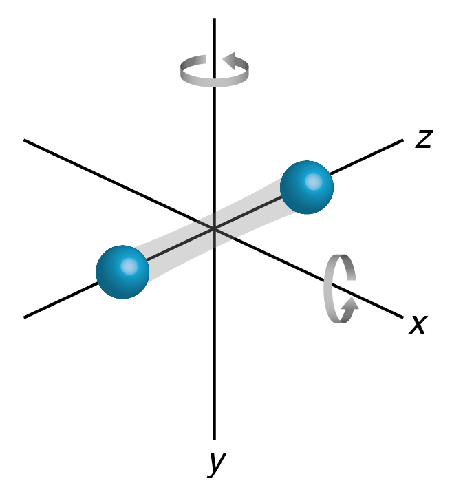
In the Section 13.5.2, we found that for an ideal gas, the average kinetic energy is given by \(\frac32 \kB T\). This is the simplest example of a much more general result from the theory of statistical physics, known as the equipartition theorem. Remember how we got the factor 3 in equation (13.21), it’s simply because each molecule can move in three different directions. We call each ‘option’ that a molecule has a degree of freedom. A single-atom molecule of an ideal gas has only one option in life: it can move, or translate, in the three cardinal directions, so it has three degrees of freedom. A diatomic ideal gas has more options, because it can also change its orientation: rotating about its long axis won’t change anything (and thus is not a degree of freedom), but rotating about an axis perpendicular to the long axis does change something. There are two such perpendicular axes, which give two additional degrees of freedom (not surprisingly, given that you also need to specify two angles to determine an orientation in space), so a diatomic molecule has three translational and two rotational degrees of freedom. The equipartition theorem states that the total internal energy of a system is directly related to the number of degrees of freedom:
Theorem 13.1 (Equipartition theorem for ideal gases)
The total internal energy of an ideal gas is given by
where \(d\) is the number of degrees of freedom.
The full equipartition theorem is even stronger than the statement given above - it can also account for systems in which there are intermolecular forces, as long as their potential energies depend quadratically on distance. Fortunately, this is the case for an important example: the potential energy of a spring, which is given by \(\frac12 C x^2\), where \(x\) is the length of the spring. This allows us to include internal vibrations in molecules in our calculations, as well as consider solids, because in both cases the links between the atoms can be modeled as springs. We will not go into more detail here, but only give the general statement:
Theorem 13.2 (Equipartition theorem)
Each quadratic term in the energy of a system contributes an amount equal to \(\frac12 \kB T\) to the internal (thermal) energy.
13.6. Problems#
Exercise 13.1 (Water and ice)
In the worked example of Example 13.1, how much ice would we have to add to bring all the water down to \(0^\circ\mathrm{C}\)?
Exercise 13.2 (Steam and water)
We add \(40.0\;\mathrm{g}\) of steam at \(100.0^\circ\mathrm{C}\) to an insulated box already containing \(200.0\;\mathrm{g}\) of water at \(50.0^\circ\mathrm{C}\). Water has a specific heat of \(4190\; \mathrm{J}/\mathrm{kg}\cdot\mathrm{K}\) and a heat of vaporization of \(2256\cdot 10^3 \; \mathrm{J}/\mathrm{kg}\).
Show that if no heat is lost to the surroundings, the final temperature of the system is \(100^\circ\mathrm{C}\).
Once the system has reached equilibrium, what is the mass of the remaining steam, and what of the remaining liquid water?
Exercise 13.3 (Evaporating boiling water)
A steel pan with a radius of \(8.0\;\mathrm{cm}\) and thickness of \(7.0\;\mathrm{mm}\) contains \(1.5\;\mathrm{L}\) of water. The thermal conductivity of steel is \(k = 46\;\mathrm{W}/(\mathrm{m}\cdot \mathrm{K})\). We put the pan on an electric stove that reaches a temperature of \(300^\circ\mathrm{C}\). Assume no heat is lost. How much time does it take to evaporate all the water once it is boiling?
Exercise 13.4 (Debye’s law for heat capacity)
The heat capacity of a material itself often depends on temperature. At very low temperatures, the heat capacity of many materials is given by Debye’s \(T^3\) law:
where \(k\) and \(\Theta\) are positive constants. For a certain material, the numerical values of the constants are \(k=2000\;\mathrm{J}/\mathrm{mol}\cdot\mathrm{K}\) and \(\Theta=280\;\mathrm{K}\). How much heat is required to raise the temperature of \(1.00\;\mathrm{mol}\) of this material from \(10.0\;\mathrm{K}\) to \(40.0\;\mathrm{K}\)?
Exercise 13.5 (The coefficient of volume expansion)
When an object or fluid is free to adjust its volume, raising its temperature will result in a thermal expansion. This expansion can be quantified by the material’s coefficient of volume expansion, defined as
Show that the coefficient of volume expansion of an ideal gas at constant pressure is the reciprocal of its temperature (in Kelvins), i.e., prove that \(\beta_\mathrm{ideal gas} = 1/T\).
The coefficient of volume expansion of water in the temperature range from \(0^\circ\mathrm{C}\) to \(20^\circ\mathrm{C}\) is given approximately by \(\beta = a + bT + cT^2\), where \(T\) is in Celsius, and \(a = -6.43 \cdot 10^{-5} (^\circ\mathrm{C})^{-1}, b = 1.70 \cdot 10^{-5} (^\circ\mathrm{C})^{-2}\), and \(c = -2.02 \cdot 10^{-7} (^\circ\mathrm{C})^{-3}\). Find the temperature at which water has its greatest density.
If a sample of water occupies 1.00000 L at \(0^\circ\mathrm{C}\), find its volume at \(12^\circ\mathrm{C}\). To answer this question, use the expression for \(\beta\) in (b) and integrate equation (13.26). For elongated objects (typically long metal rods), often only the expansion in the elongated direction is relevant, and we define the coefficient of linear expansion \(\alpha\):
(13.27)#\[\alpha = \frac{1}{L} \frac{\mathrm{d}L}{\mathrm{d}T}.\]Show that coefficient of volume expansion and that of linear expansion for a uniform material are related as \(\beta = 3 \alpha\). Hint: consider a cube with sides \(a\).
Exercise 13.6 (An ideal gas in a cylindrical tube)
Consider a cylindrical tube of length \(L\), which contains an ideal gas, initially at \(T=T_0\) and atmospheric pressure \(p_0\). The tube is divided into two initially equal-size chambers by a wall that can slide without friction along the length of the tube. The left chamber is heated to a high temperature \(T_\mathrm{f}\).
What will be the position of the wall (as measured from the left side of the cylinder) if we keep the temperature on the other side constant? If we do not regulate the temperature, the gas in the right chamber heats up due to compression. After a while, the system has reached equilibrium; we measure the final temperature on the right to be \(T_1\).
What is the position of the wall in this case?
How large is then the pressure on the left and right side of the wall?
Exercise 13.7 (Maxwell distribution for the speeds of molecules in an ideal gas)
In Section 13.5.3, we introduced the Maxwell distribution (equation (13.23)) for the distribution of the speeds of the molecules in an ideal gas.
The central limit theorem states that for any large enough collection of independent, identically distributed stochastic variables, the distribution of the normalized sum of all variables tends to a Gaussian distribution. Argue why the \(x\)-, \(y\)- and \(z\)-components of the velocities of the molecules in an ideal gas are indeed independent and identically distributed.
The Gaussian distribution function for a stochastic variable \(x\) with mean \(\mu\) and standard deviation \(\sigma\) is given by
\[f(x) = \frac{1}{\sqrt{2 \pi}\sigma} \exp\left[-\frac12 \left(\frac{x-\mu}{\sigma}\right)^2 \right].\]Argue why, for each of the components of the velocity, the mean should be zero.
Using what we know about the mean speed of the particles, find the standard deviation \(\sigma\) of the velocities.