
2. Forces#
2.1. Newton’s laws of motion#
As described in Section 1, classical mechanics is based on a set of axioms, which in turn are based on (repeated) physical observations. In order to formulate the first three axioms, we will need to first define three quantities: the (instantaneous) velocity, acceleration and momentum of a particle. If we denote the position of a particle as \(\bm{x}(t)\), indicating a vector[1] quantity with the dimension of length that depends on time, we define its velocity as the time derivative of the position:
Note that we use an overdot to indicate a time derivative. We will use this convention throughout this book. The acceleration is the time derivative of the velocity, and thus the second derivative of the position:
Finally, the momentum of a particle is its mass times its velocity:
We are now ready to give our next three axioms. You may have encountered them before; they are known as Newton’s three laws of motion.
Axiom 2.1 (Newton’s first law of motion)
As long as there is no external action, a particle’s velocity will remain constant.
Note that the first law includes particles at rest, i.e., \(\bm{v} = 0\). We will define the general ‘external action’ as a force, therefore a force is now anything that can change the velocity of a particle. The second law quantifies the force.
Isaac Newton (1642-1727)
Isaac Newton (1642-1727) was a British physicist, astronomer and mathematician, who is widely regarded as one of the most important scientists in history. Newton was a professor at Cambridge from 1667 till 1702, where he held the famous Lucasian chair in mathematics. Newton invented infinitesimal calculus to be able to express the laws of mechanics that now bear his name (Section 2.1) in mathematical form. He also gave a mathematical description of gravity (equation (2.9)), from which he could derive Kepler’s laws of planetary motion (Section 6.4). In addition to his work on mechanics, Newton made key contributions to optics and invented the reflection telescope, which uses a mirror rather than a lens to gather light. Having retired from his position in Cambridge, Newton spent most of the second half of his life in London, as warden and later master of the Royal Mint, and president of the Royal Society.
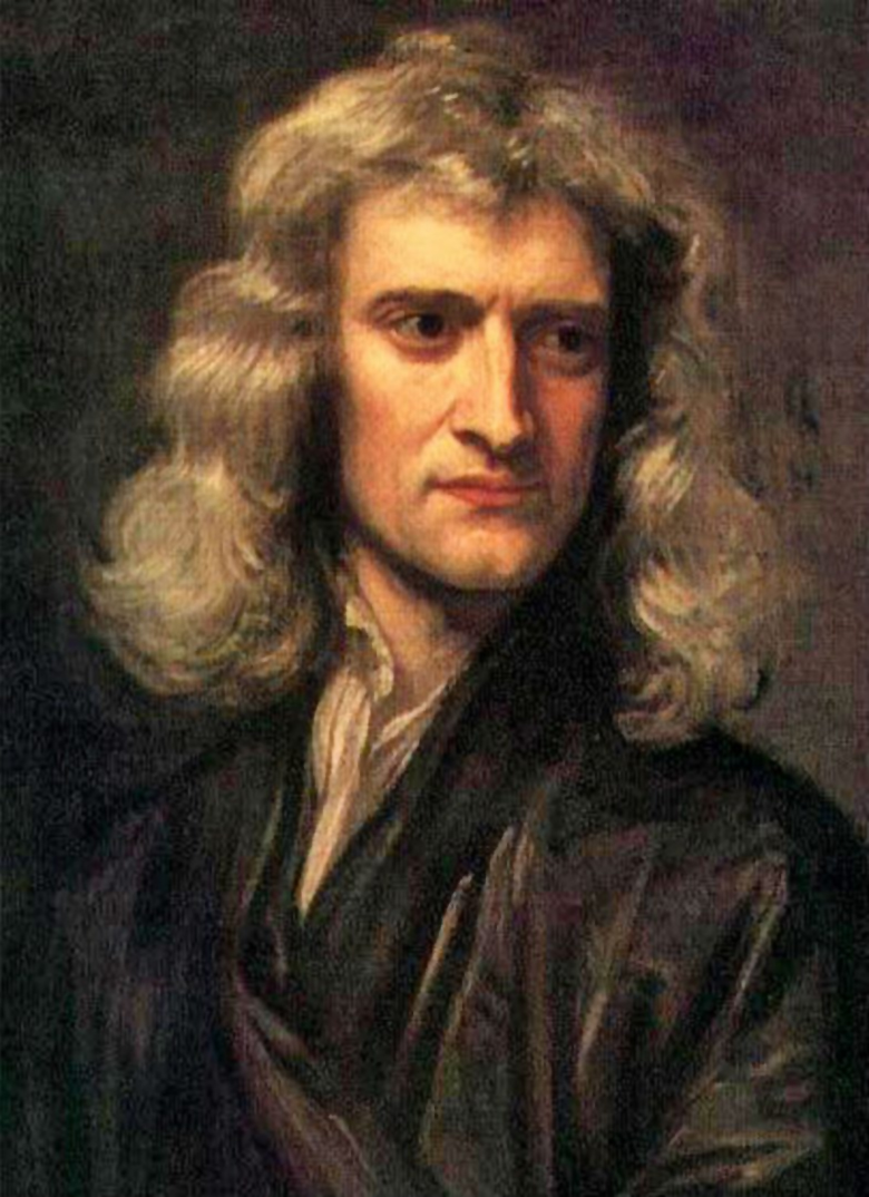
Fig. 2.1 Portrait of Isaac Newton by Godfrey Kneller (1689) [2].#
Axiom 2.2 (Newton’s second law of motion)
If there is a net force acting on a particle, then its instantaneous change in momentum due to that force is equal to that force:
Now, since \(\bm{p} = m\bm{v}\) and \(\bm{a} = \mathrm{d}\bm{v}/\mathrm{d}t\), if the mass is constant we can also write (2.4) as \(\bm{F} = m \bm{a}\), or
which is the form we will use most. Based on the second law, we see that a force has the physical dimension of a mass times a length divided by a time squared, for which we’ll use a ‘dimensional short-hand’ \(F = MLT^{-2}\). Likewise, we define a unit, the Newton (\(\mathrm{N}\)), as a kilogram times a meter per second squared: \(\mathrm{N} = \mathrm{kg} \cdot \mathrm{m} / \mathrm{s}^2\). Therefore, in principle Newton’s second law of motion can also be used to measure forces, though we will often use it the other way around, and calculate changes in momentum due to a known force.
Note how Newton’s first law follows from the second: if the force is zero, there is no change in momentum, and thus (assuming constant mass) a constant velocity. Note also that although the second law gives us a quantification of the force, by itself it will not help us achieve much, as we at present have no idea what the force is (though you probably have some intuitive ideas from experience) - for that we will use the force laws of the next section. Before we go there, there is another important observation on the nature of forces in general.
Axiom 2.3 (Newton’s third law of motion)
If a body exerts a force \(\bm{F}_1\) on a second body, the second body exerts an equal but opposite force \(\bm{F}_2\) on the first, i.e., the forces are equal in magnitude but opposite in direction:
2.2. Force laws#
Newton’s second law of motion tells us what a force does: it causes a change in momentum of any particle it acts upon. It does not tell us where the force comes from, nor does it care - which is a very useful feature, as it means that the law applies to all forces. However, we do of course need to know what the force is, so we need some rule to determine it independently. This is where the force laws come in.
Robert Hooke (1635-1703)
Robert Hooke (1635-1703) was a British all-round natural scientist and architect. He discovered the force law named after him in 1660, which he published first as an anagram: ‘ceiiinosssttuv’, so he could claim the discovery without actually revealing it (a fairly common practice at the time); he only provided the solution in 1678: ‘ut tensio, sic vis’ (‘as the extension, so the force’). Hooke made many contributions to the development of microscopes, using them to reveal the structure of plants, coining the word ‘cell’ for their basic units. Hooke was the curator of experiments of England’s Royal Society for over 40 years, combining this position with a professorship in geometry and the job of surveyor of the city of London after the great fire of 1666. In the latter position he got a strong reputation for his hard work and great honesty. At the same time, he was frequently at odds with his contemporaries Isaac Newton and Christiaan Huygens; it is not unlikely that they all independently developed similar notions on, among others, the inverse-square law of gravity.
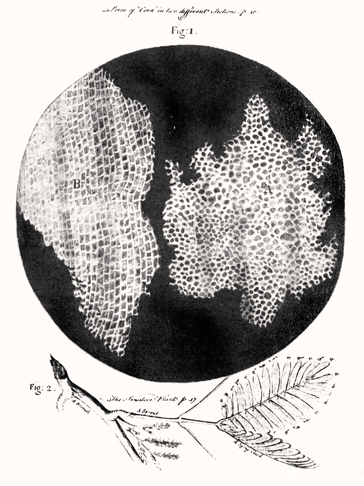
Fig. 2.2 Drawing of the cell structure of cork by Hooke, from his 1665 book Micrographia [3]. No portraits of Hooke survive.#
2.2.1. Springs: Hooke’s law#
One very familiar example of a force is the spring force: you need to exert a force on something to compress it, and (in accordance with Newton’s third law), if you press on something you’ll feel it push back on you. The simplest possible object that you can compress is an ideal spring, for which the force necessary to compress it scales linearly with the compression itself. This relation is known as Hooke’s law:
where \(\bm{x}\) is now the displacement (from rest) and \(k\) is the spring constant, measured in newtons per meter. The value of \(k\) depends on the spring in question - stiffer springs having higher spring constants.
Hooke’s law gives us another way to measure forces. We have already defined the unit of force using Newton’s second law of motion, and we can use that to calibrate a spring, i.e., determine its spring constant, by determining the displacement due to a known force. Once we have \(k\), we can simply measure forces by measuring displacements - this is exactly what a spring scale does.
2.2.2. Gravity: Newton’s law of gravity#
A second and probably even more familiar example is force due to gravity. Anything that has mass attracts everything else that has mass, and since the Earth is very massive, it attracts all objects in the space around you, including yourself. Since the force of gravity is weak, you won’t feel the pull of your book, but since the Earth is so massive, you do feel its pull. Therefore if you let go of something, it will be accelerated towards the Earth due to its attracting gravitational force. As demonstrated by Galilei (and some guys in spacesuits on a rock we call the moon[4]), the acceleration of any object due to the force of gravity is the same, and thus the force exerted by the Earth on any object equals the mass of that object times this acceleration, which we call \(\bm{g}\):
Because the Earth’s mass is not uniformly distributed, the magnitude \(g\) of \(\bm{g}\) varies slightly from place to place, but to good approximation equals \(9.81\,\mathrm{m}/\mathrm{s}^2\). It always points down.
Although equation (2.8) for local gravity is handy, its range of application is limited to everyday objects at everyday altitudes - say up to a couple thousand kilograms and a couple kilometers above the surface of the Earth, which is tiny compared to Earth’s mass and radius. For larger distances and bodies with larger mass - say the Earth-Moon or Earth-Sun systems - we need something else, namely Newton’s law of gravitation between two bodies with masses \(m_1\) and \(m_2\) and a distance \(r\) apart:
where \(\bm{\hat{r}}\) is the unit vector pointing along the line connecting the two masses, and the proportionality constant \(G = 6.67 \cdot 10^{-11} \; \mathrm{N} \cdot \mathrm{m}^2 / \mathrm{kg}^2\), which is known as the gravitational constant (or Newton’s constant). The minus sign indicates that the force is attractive. Equation (2.9) allows you to actually calculate the gravitational pull that your book exerts on you, and understand why you don’t feel it. It also lets you calculate the value of \(g\) - simply substitute the mass and radius of the Earth, so \(g = G M_\mathrm{E} / R_\mathrm{E}^2\). If you wish to know the value of \(g\) on any other celestial body, you can put in its particulars, and compare with Earth. You’ll find you’d ‘weigh’ \(3\) times less on Mars and \(6\) times less on the Moon. Most of the time we can safely assume the Earth is flat and use (2.8), but in particular for celestial mechanics and when considering satellites we’ll need to use (2.9).
Galileo Galilei (1564-1642)
Galileo Galilei (1564-1642) was an Italian physicist and astronomer, who is widely regarded as one of the founding figures of modern science. Unlike classical philosophers, Galilei championed the use of experiments and observations to validate (or disprove) scientific theories, a practice that is now the cornerstone of the scientific method. He pioneered the use of the telescope (newly invented at the time) for astronomical observations, leading to his discovery of mountains on the moon an the four largest moons of Jupiter (now known as the Galilean moons in his honor). On the theoretical side, Galilei argued that Aristotle’s argument that heavy objects fall faster than light ones is incorrect, and that the acceleration due to gravity is equal for all objects (equation (2.8)). Galilei also strongly advocated the heliocentric worldview introduced by Copernicus in 1543, as opposed to the widely-held geocentric view. Unfortunately, the Inquisition thought otherwise, leading to his conviction for heresy with a sentence of life-long house arrest in 1633, a position that was only recanted by the church in 1995.
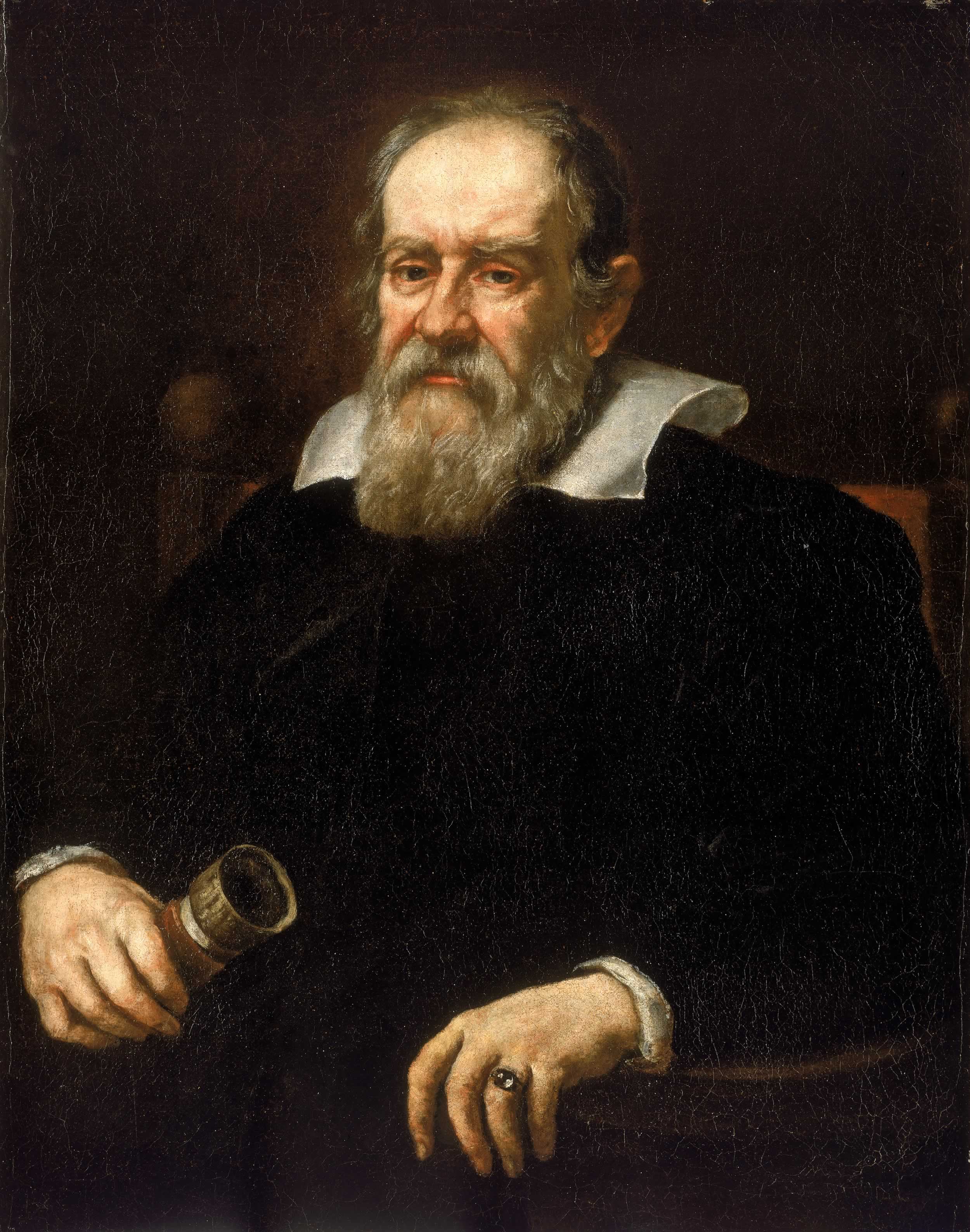
Fig. 2.3 Portrait of Galileo Galilei by Justus Sustermans (1636) [5].#
2.2.3. Electrostatics: Coulomb’s law#
Just like two masses interact due to the gravitational force, two charged objects interact via Coulomb’s force. Because charge has two possible signs, Coulomb’s force can both be attractive (between opposite charges) and repulsive (between identical charges). Its mathematical form strongly resembles that of Newton’s law of gravity:
where \(q_1\) and \(q_2\) are the signed magnitudes of the charges, \(r\) is again the distance between them, and \(k_\mathrm{e} = 8.99 \cdot 10^9\;\mathrm{N} \cdot \mathrm{m}^2/\mathrm{C}^{2}\) is Coulomb’s constant. For everyday length and force scales, Coulomb’s force is much larger than the force of gravity.
2.2.4. Friction and drag#
Why did it take the genius of Galilei and Newton to uncover Newton’s first law of motion? Because everyday experience seems to contradict it: if you don’t exert a force, you won’t keep moving, but gradually slow down. You know of course why this is: there’s drag and friction acting on a moving body, which is why it’s much easier (though not necessarily handier) for a car to keep moving on ice than on a regular tarmac road (less friction on ice), and why walking through water is so much harder than walking through air (more drag in water). The medium in which you move can exert a drag force on you, and the surface over which you move exerts friction forces. These of course are the forces responsible for slowing you down when you stop exerting force yourself, so the first law doesn’t apply, as there are forces acting.
For low speeds, the drag force typically scales linearly with the velocity of the moving object. Drag forces for objects moving through a (fluid) medium moreover depend on the properties of the medium (its viscosity \(\eta\)) and the cross-sectional area of the moving object. For a sphere of radius \(R\) moving at velocity \(\bm{v}\), the drag force is given by Stokes’ law:
The more general version for an object of arbitrary shape is \(\bm{F}_\mathrm{d} = -\zeta \bm{v}\), where \(\zeta\) is a proportionality constant. Stokes’ law breaks down at high velocities, for which the drag force scales quadratically with the speed:
where \(\rho\) is the density of the fluid, \(A\) the cross-sectional area of the object, \(v\) it’s speed, and \(c_\mathrm{d}\) it’s dimensionless drag coefficient, which depends on the object’s shape and surface properties. Typical values for the drag coefficient are \(1.0\) for a cyclist, \(1.2\) for a running person, \(0.48\) for a Volkswagen Beetle, and \(0.19\) for a modern aerodynamic car. The direction of the drag force is always opposite to that of the motion.
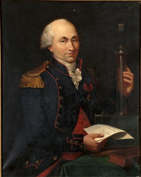
Charles-Augustin de Coulomb (1736-1806)
Charles-Augustin de Coulomb (1736-1806) was a French physicist and military engineer. For most of his working life, Coulomb served in the French army, for which he supervised many construction projects. As part of this job, Coulomb did research, first in mechanics (leading to his law of kinetic friction, equation (2.13)), and later in electricity and magnetism, for which he discovered that the force between charges (and those between magnetic poles) drops off quadratically with their distance (equation (2.10)). Near the end of his life, Coulomb participated in setting up the SI system of units.
Frictional forces are due to two surfaces sliding past each other. It should come as no surprise that the direction of the frictional force is opposite that of the motion, and its magnitude depends on the properties of the surfaces. Moreover, the magnitude of the frictional force also depends on how strongly the two surfaces are pushed against each other - i.e., on the forces they exert on each other, perpendicular to the surface. These forces are of course equal (by Newton’s third law) and are called normal forces, because they are normal (that is, perpendicular) to the surface. If you stand on a box, gravity exerts a force on you, pulling you down, which you ‘transfer’ to a force you exert on the top of the box, and causes an equal but opposite normal force exerted by the top of the box on your feet. If the box is tilted, the normal force is still perpendicular to the surface (it remains normal), but is no longer equal in magnitude to the force exerted on you by gravity. Instead, it will be equal to the component of the gravitational force along the direction perpendicular to the surface (see Fig. 2.6). We denote normal forces as \(\bm{F}_n\). Now according to the Coulomb friction law (not to be confused with the Coulomb force between two charged particles), the magnitude of the frictional force between two surfaces satisfies
Here \(\mu\) is the coefficient of friction, which of course depends on the two surfaces, but also on the question whether the two surfaces are moving with respect to each other or not. If they are not moving, i.e., the configuration is static, the appropriate coefficient is called the coefficient of static friction and denoted by \(\mu_s\). The actual magnitude of the friction force will be such that it balances the other forces (more on that in Section 2.4). Equation (2.13) tells us that this is only possible if the required magnitude of the friction force is less than \(\mu_s F_n\). When things start moving, the static friction coefficient is replaced by the coefficient of kinetic friction \(\mu_k\), which is usually smaller than \(\mu_s\). For kinetic friction the inequality in equation (2.13) gets replaced by an equals sign, and we have \(F_f = \mu_k F_n\).
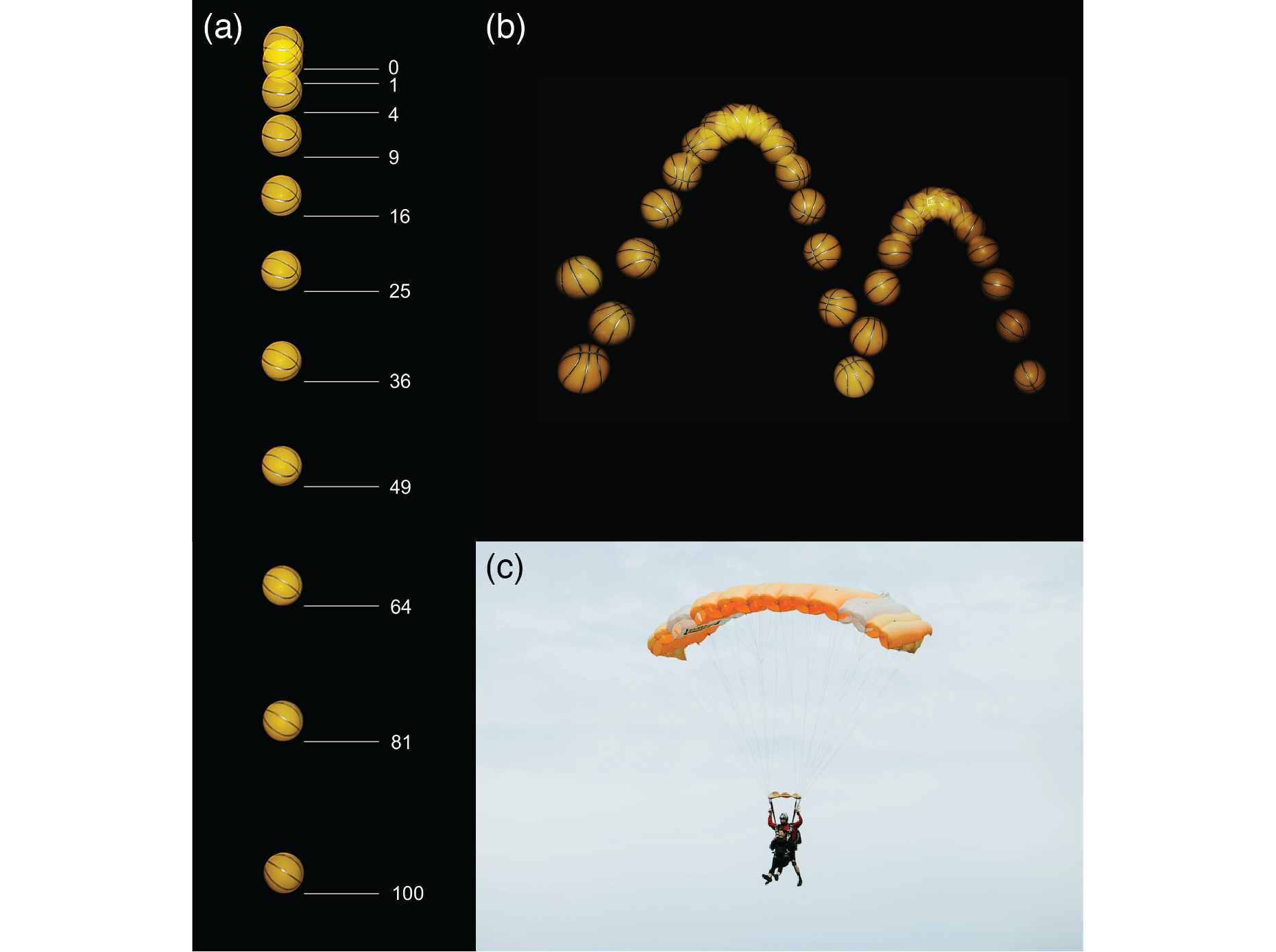
Fig. 2.5 Dropping under the force of gravity. (a and b) A ball released from rest drops with a constant acceleration, resulting in a constantly increasing velocity. Images in (a) are taken every \(0.05\;\mathrm{s}\); distances are multiples of \(12\;\mathrm{mm}\). In (b), the trajectory of the ball resulting from repeated bounces is shown with intervals of \(0.04\;\mathrm{s}\) [7], CC BY-SA 3.0. (c) Paragliders need to balance the force of gravity and that of drag to stop accelerating and fall at a continuous speed (known as their terminal velocity) [8], CC BY-SA 3.0.#
2.3. Equations of motion#
Now that we have set our axioms - Newton’s laws of motion and the various force laws - we are ready to start combining them to get useful results, things that are not put into the axioms but follow from them. The first thing we can do is write down equations of motion: an equation that describes the motion of a particle due to the action of a certain type of force. For example, suppose you take a rock of a certain mass \(m\) and let go of it at some height \(h\) above the ground, what will happen? Once you’ve let go of the rock, there is only one force acting on the rock, namely Earth’s gravity, and we are well within the regime where equation (2.8) applies, so we know the force. We also know that this net force will result in a change of momentum (equation (2.4)), which, because the rock won’t lose any mass in the process of falling, can be rewritten as (2.5). By equating the forces we arrive at an equation of motion for the rock, which in this case is very simple:
We immediately see that the mass of the rock doesn’t matter (Galilei was right! - though of course he was in our set of axioms, because we arrived at them by assuming he was right). Less trivially, equation (2.14) is a second-order differential equation for the motion of the rock, which means that in order to find the actual motion, we need two initial conditions - which in our present example are that the rock starts at height \(h\) and zero velocity.
Equation (2.14) is essentially one-dimensional - all motion occurs along the vertical line. Solving it is therefore straightforward - you simply integrate over time twice. The general solution is:
which with our boundary conditions becomes
where \(g\) is the magnitude of \(\bm{g}\) (which points down, hence the minus sign). Of course equation (2.16) breaks down when the rock hits the ground at \(t = \sqrt{2h/g}\), which is easily understood because at that point gravity is no longer the only force acting on it.
We can also immediately write down the equation of motion for a mass on a spring (without gravity), in which the net force is given by Hooke’s law. Equating that force to the net force in Newton’s second law of motion gives:
Of course, we find another second-order differential equation, so we again need the initial position and velocity to specify a solution. The general solution of (2.17) is a combination of sines and cosines, with a frequency \(\omega = \sqrt{k/m}\) (as we already know from the dimensional analysis in Section 1.2):
We’ll study this case in more detail in Section 8.1.
In general, the force in Newton’s second law may depend on time and position, as well as on the first derivative of the position, i.e., the velocity. For the special case that it depends on only one of the three variables, we can write down the solution formally, in terms of an integral over the force. These formal solutions are given in Section 2.6. To see how they work in practice, let’s consider a slightly more involved problem, that of a stone falling with drag.
Example 2.1 (falling stone with drag)
Suppose we have a spherical stone of radius \(a\) that you drop from a height \(h\) at \(t = 0\). At what time, and with which velocity, will the stone hit the ground? We already solved this problem in the simple case without drag above, but now let’s include drag. There are then two forces acting on the stone: gravity (pointing down) with magnitude \(mg\), and drag (pointing in the direction opposite the motion, in this case up) with magnitude \(6 \pi \eta a v = b v\), as given by Stokes’ law (equation (2.11)). Our equation of motion is now given by (with \(x\) as the height of the particle, and the downward direction as positive):
We see that our force does not depend on time or position, but only on velocity - so we have case 3 of Section 2.6. We could invoke either equation (2.33) or (2.34) to write down a formal solution, but there is an easier way, which will allow us to evaluate the relevant integrals without difficulty. Since our equation of motion is linear, we know that the sum of two solutions is again a solution. One of the terms on the right hand side of equation (2.19) is constant, which means that our equation is not homogeneous (we can rewrite it to \(m \ddot{x} + b \dot{x} = m g\) to see this), so it’s useful to split our solution in a homogeneous and a particular part. Rewriting our equation in terms of \(v = \dot{x}\) instead of \(x\), we get \(m \dot{v} + b v = m g\), from which we can immediately get a particular solution: \(v_\mathrm{p} = m g / b\), as the time derivative of this constant \(v_\mathrm{p}\) vanishes. Subtracting \(v_\mathrm{p}\), we are left with a homogeneous equation: \(m \dot{v}_\mathrm{h} + b v_\mathrm{h}\), which we now solve by separation of variables. First we write \(\dot{v}_\mathrm{h} = \mathrm{d}v_\mathrm{h} / \mathrm{d}t\), then re-arrange so that all factors containing \(v_\mathrm{h}\) are on one side and all factors containing \(t\) are on the other, which gives \(-(m/b) (1/v_\mathrm{h}) \mathrm{d}v_\mathrm{h} = \mathrm{d}t\). We can now integrate to get:
which is an example of equation (2.33). After rearranging and setting \(t_0 = 0\):
Note that this homogeneous solution fits our intuition: if there is no extra force on the particle, the drag force will slow it down exponentially. Also note that we didn’t set \(v_0 = 0\), as the homogeneous solution does not equal the total solution. Instead \(v_0\) is an integration constant that we’ll need to set once we’ve written down the full solution, which is:
Now setting \(v(0) = 0\) gives \(v_0 = -mg/b\), so
To get \(x(t)\), we simply integrate \(v(t)\) over time, to get:
We can find when the stone hits the ground by setting \(x(t) = h\) and solving for \(t\); we can find how fast it is going at that point by substituting that value of \(t\) back into \(v(t)\).
2.4. Multiple forces#
In the examples in Section 2.3 there was only a single force acting on the particle of interest. Usually there will be multiple forces acting at the same time, not necessarily pulling in the same direction. This is where vectors come into play.
Suppose you put a book on a table. Earth’s gravity pulls it down with a force of magnitude \(F_g\). Consequently the book exerts a normal force down on the table with the same magnitude, and the table reciprocates with an identical but oppositely directed normal force of magnitude \(F_n = F_g\). Now suppose you push against the book from the side with a force of magnitude \(F\). As we’ve seen in Section 2.2, there will then be a friction force between the book and the table in the opposite direction, which, as long as it doesn’t exceed \(\mu_s F_n\), equals the force you push with. However, once \(F\) is larger than \(\mu_s F_n\), there will be a net force acting on the book. It is the net force that we substitute into Newton’s second law, and from which the book will get a net acceleration.
In the situation described above, things are still simple - you get the net force by subtracting the kinetic friction \(F_f = \mu_f F_n\) from the force \(F\) you exert on the book, because these are horizontal and thus perpendicular to the vertical normal and gravitational forces. But what happens if you lift the table on one end, so that it becomes slanted? To help organize our thoughts, we’ll draw a free body diagram, shown in Fig. 2.6. Gravity still acts downward, and the mass of the book stays the same, so \(\bm{F}_g\) doesn’t change. However, the orientation of the contact plane between the book and table does change, so the normal force (remember, normal to the surface) changes as well. Its direction will remain perpendicular to the surface, and as long as you don’t push on the book (or push along the surface only), the only other force having a component perpendicular to the surface is gravity, so the magnitude of the normal force better be equal to that (otherwise the book would either spontaneously start to float, or fall through the table). You can find this component by decomposing the gravitational force along the directions perpendicular and parallel to the slanted surface. The remaining component of the gravitational force points downward along the surface of the table, and is comparable to the force you were exerting on the book when the table was horizontal. Up to some point this downward force is balanced by a static frictional force, but once it gets too large (because the slant angle of the table gets too large), friction reaches its maximum and gravity results in a net force on the book, which will start to slide down (as you no doubt guessed already).

Fig. 2.6 Free body diagram of the forces acting on a book on a slanted table. Gravity always points down, normal forces are always perpendicular to the surface, and frictional forces always parallel to the surface. The force of gravity can be decomposed in directions perpendicular and parallel to the surface as well.#

2.5. Statics#
When multiple forces act on a body, the (vector) sum of those forces gives the net force, which is the force we substitute in Newton’s second law of motion to get the equation of motion of the body. If all forces add up to zero, there will be no acceleration, and the body retains whatever velocity it had before. Statics is the study of objects that are neither currently moving nor experiencing a net force, and thus remain stationary. You might expect that this study is easier than the dynamical case when bodies do experience a net force, but that just depends on context. Imagine, for example, a jar filled with marbles: they aren’t moving, but the forces acting on the marbles are certainly not zero, and also not uniformly distributed.
Even if there is no net force, there is no guarantee that an object will exhibit no motion: if the forces are distributed unevenly along an extended object, it may start to rotate. Rotations always happen around a stationary point, known as the pivot. Only a force that has a component perpendicular to the line connecting its point of action to the pivot (the arm) can make an object rotate. The corresponding angular acceleration due to the force depends on both the magnitude of that perpendicular component and the length of the arm, and is known as the moment of the force or the torque \(\bm{\tau}\). The magnitude of the torque is therefore given by \(F r \sin\theta\), where \(F\) is the magnitude of the force, \(r\) the length of the arm, and \(\theta\) the angle between the force and the arm. If we write the arm as a vector \(\bm{r}\) pointing from the pivot to the point where the force acts, we find that the magnitude of the torque equals the cross product of \(\bm{r}\) and \(\bm{F}\):
The direction of rotation can be found by the right-hand rule from the direction of the torque: if the thumb of your right hand points along the direction of \(\bm{\tau}\), then the direction in which your fingers curve will be the direction in which the object rotates due to the action of the corresponding force \(\bm{F}\).
We will study rotations in detail in Section 5. For now, we’re interested in the case where there is no motion, neither linear nor rotational, which means that the forces and torques acting on our object must satisfy the stability condition: for an extended object to be stationary, both the sum of the forces and the sum of the torques acting on it must be zero.
Example 2.2 (Suspended sign)
A sign of mass \(M\) hangs suspended from a rod of mass \(m\) and length \(L\) in a symmetric way and such that the centers of mass of the sign and rod align nicely (Fig. 2.7a). One end of the rod is anchored to a wall directly, while the other is supported by a wire with negligible mass that is attached to the same wall a distance \(h\) above the anchor. (a) If the maximum tension the wire can support is \(T\), find the minimum value of \(h\). (b) For the case that the tension in the wire equals the maximum tension, find the force (magnitude and direction) exerted by the anchor on the rod.

Fig. 2.7 A suspended sign (example of a calculation in statics). (a) Problem setting. (b) Free-body diagram.#
Solution
We first draw a free-body diagram, Fig. 2.7b. Force balance on the sign tells us that the tensions in the two lower wires add up to the gravitational force on the sign. The rod is stationary, so we know that the sum of the torques on it must vanish. To get torques, we first need a pivot; we pick the point where the rod is anchored to the wall. We then have three forces contributing a clockwise torque, and one contributing a counterclockwise torque. We’re not told exactly where the wires are attached to the rod, but we are told that the configuration is symmetric and that the center of mass of the sign aligns with that of the rod. Let the first wire be a distance \(\alpha L\) from the wall, and the second a distance \((1-\alpha)L\). The total (clockwise) torque due to the gravitational force on the sign and rod is then given by:
\[\tau_\mathrm{z} = \frac12 m g L + \frac12 M g \alpha L + \frac12 M g (1-\alpha) L = \frac12 (m+M)gL.\]The counterclockwise torque comes from the tension in the wire, and is given by
\[\tau_\mathrm{wire} = F_\mathrm{T} \sin\theta L = F_\mathrm{T} (h/\sqrt{h^2+L^2}) L.\]Equating the two torques allows us to solve for \(h\) as a function of \(F_\mathrm{T}\), as requested, which gives:
\[h^2 = \left(\frac12 \frac{(m+M)g}{F_\mathrm{T}} \right)^2 (h^2 + L^2) \quad \rightarrow \quad h = \frac{(m+M)gL}{\sqrt{4 F_\mathrm{T}^2 - (m+M)^2 g^2}}.\]We find the minimum value of \(h\) by substituting \(F_\mathrm{T} = T_\mathrm{max}\).
As the rod is stationary, all forces on it must cancel. In the horizontal direction, we have the horizontal component of the tension, \(T_\mathrm{max} \cos\theta\) to the left, which must equal the horizontal component of the force exerted by the wall, \(F_\mathrm{w} \cos\phi\). In the vertical direction, we have the gravitational force and the two forces from the wires on which the sign hangs in the downward direction, and the vertical component of the tension in the wire in the upward direction, the sum of which must equal the vertical component of the force exerted by the wall (which may point either up or down). We thus have
\[\begin{split}\begin{align*} F_\mathrm{w} \cos\phi &= T_\mathrm{max} \cos\theta, \\ F_\mathrm{w} \sin\phi &= (m+M)g + T_\mathrm{max} \sin\theta, \end{align*}\end{split}\]where \(\tan\theta = h/L\) and \(h\) is given in the answer to (a). We find that
\[\begin{split}\begin{align*} F_\mathrm{w}^2 &= T_\mathrm{max}^2 + 2 (m+M)g T_\mathrm{max} \sin\theta + (m+M)^2 g^2, \\ \tan \phi &= \frac{T_\mathrm{max} \cos\theta}{(m+M)g + T_\mathrm{max} \sin\theta}. \end{align*}\end{split}\]Note that the above expressions give the complete answer (magnitude and direction). We could eliminate \(h\) and \(\theta\), but that’d just be algebra, leading to more complicated expressions, and not very useful in itself. If we’d been asked to calculate the height or force for any specific values of \(M\), \(m\), and \(L\), we could get the answers easily by substituting the numbers in the expressions given here.
2.6. Solving the equations of motion in three special cases*#
In Section 2.3 we saw some examples of equations of motion originating from Newton’s second law of motion. For the quite common case that the mass of our object of interest is constant, its trajectory will be given as the solution of a second-order ordinary differential equation, with time as our variable. In general, the force in Newton’s second law may depend on time and position, as well as on the first derivative of the position, i.e., the velocity. In one dimension, we thus have
We cannot solve equation (2.26) for a general function \(F\). However, in each of the special cases that the force depends on only one of the three variables, we can find a general solution, albeit as an integral over the force, which we may or may not be able to calculate explicitly.
2.6.1. Case 1: \(F = F(t)\)#
If the force only depends on time, we can solve equation (2.26) by direct integration. Using that \(v = \dot{x}\), we have \(m \dot{v} = F(t)\), which we integrate to find
where at the initial time \(t=t_0\) the object has velocity \(v=v_0\). We can now find the position by integrating the velocity:
2.6.2. Case 2: \(F = F(x)\)#
If the force depends only on the position in space (as is the case for the harmonic oscillator), we cannot integrate over time, as to do so we would already need to know \(x(t)\). Instead, we invoke the chain rule to rewrite our differential equation as an equation in which the position is our variable. We have:
and so our equation of motion becomes
which we again solve by direct integration:
To get \(x(t)\), we use the relation that \(\mathrm{d}x/\mathrm{d}t = v(x)\). Separation of variables gives \(\mathrm{d}x / v(x) = \mathrm{d}t\), which we can integrate to get
which gives us \(t(x)\). In principle we can invert this expression to give us \(x(t)\), although in practice this may not be easy.
2.6.3. Case 3: \(F = F(v)\)#
If the force depends only on the velocity, there are two ways we can proceed. We can write the equation of motion as \(m \mathrm{d}v / \mathrm{d} t = F(v)\) and use separation of variables to get:
from which we can get \(v(t)\) after inverting, and \(x(t)\) after integrating \(v(t)\) as in equation (2.28). Alternatively, we could again rewrite our equation of motion as an equation in space instead of time, and arrive at:
From equation (2.34) we can get \(v(x)\) by inverting, and \(x(t)\) from equation (2.32). Note that equation (2.34) does not give us \(x(t)\) directly, as \(x\) is the variable in that equation.
Example 2.3 (velocity of the harmonic oscillator)
It may seem that what we’ve done so far in this section has hardly helped matters: the ‘solutions’ we found contain integrals and often need to be inverted to get our desired function \(x(t)\) (or, depending on the problem we’re studying, \(v(t)\) or \(v(x)\)). To show you how these solutions may be useful, let’s consider a specific example: a harmonic oscillator, consisting of a mass on a Hookean spring, with \(F = F(x) = -k x\). We already wrote down the equation of motion (2.17) and its general solution (2.18). The general solution can be found through the substitution of exponentials, as we’ll do in Section 8.1. However, we can also learn something useful from writing the equation of motion in the form (2.30). Its solution, formally given by equation (2.31), can be calculated explicitly for our force as
which gives
for \(v(x)\). Although \(x(t)\) and \(v(t)\) are more easily obtained from the solution given in equation (2.18), that solution will not give you \(v(x)\), and deriving it is tricky. Here we get it almost for free. Moreover, as you have probably noted, equation (2.35) relates the kinetic to the potential energy of the harmonic oscillator - a special case of conservation of energy, which we’ll discuss in the next chapter.
2.7. Problems#
Exercise 2.1 (Terminal velocity)
The terminal velocity is the maximum (constant) velocity a dropping object reaches. In this problem, we use equation (2.12) for the drag force.
Use dimensional analysis to relate the terminal velocity of a falling object to the various relevant parameters.
Estimate the terminal velocity of a paraglider (Fig. 2.5c).
Use the concept of terminal velocity to predict whether a mouse (without parachute) is likely to survive a fall from a high tower.
Exercise 2.2 (Sticky rice)
When you cook rice, some of the dry grains always stick to the measuring cup. A common way to get them out is to turn the measuring cup upside-down and hit the bottom (now on top) with your hand so that the grains come off [9].
Explain why static friction is irrelevant here.
Explain why gravity is negligible.
Explain why hitting the cup works, and why its success depends on hitting the cup hard enough.
Exercise 2.3 (Parabolic trajectory with maximum area)
A ball is thrown at speed \(v\) from zero height on level ground. We want to find the angle \(\theta\) at which it should be thrown so that the area under the trajectory is maximized.
Sketch of the trajectory of the ball.
Use dimensional analysis to relate the area to the initial speed \(v\) and the gravitational acceleration \(g\).
Write down the \(x\) and \(y\) coordinates of the ball as a function of time.
Find the total time the ball is in the air.
The area under the trajectory is given by \(A = \int y \mathrm{d}x\). Make a variable transformation to express this integral as an integration over time.
Evaluate the integral. Your answer should be a function of the initial speed \(v\) and angle \(\theta\).
From your answer at (f), find the angle that maximizes the area, and the value of that maximum area. Check that your answer is consistent with your answer at (b).
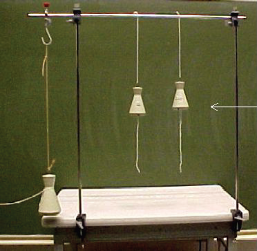
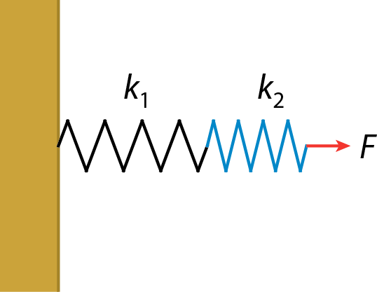
Exercise 2.4 (Springs in series)
If a mass \(m\) is attached to a spring, its period of oscillation is \(T\). If two such springs are connected end to end, and the same mass m is attached, find the new period \(T'\), in terms of the old period \(T\).
Exercise 2.5 (Two sliding blocks)
Two blocks, of mass \(m\) and \(2m\), are connected by a massless string and slide down an inclined plane at angle \(\theta\). The coefficient of kinetic friction between the lighter block and the plane is \(\mu\), and that between the heavier block and the plane is \(2\mu\). The lighter block leads.
Find the magnitude of the acceleration of the blocks.
Find the tension in the taut string.
Exercise 2.6 (Drag force on a boat)
A 1000 kg boat is traveling at 100 km/h when its engine is shut off. The magnitude \(F_\mathrm{d}\) of the drag force between the boat and the water is proportional to the speed \(v\) of the boat, with a drag coefficient \(\zeta = 70\;\mathrm{N}\cdot\mathrm{s}/\mathrm{m}\). Find the time it takes the boat to slow to 45 km/h.
Exercise 2.7 (Two attracting particles)
Two particles on a line are mutually attracted by a force \(F = - a r\), where \(a\) is a constant and \(r\) the distance of separation. At time \(t = 0\), particle A of mass \(m\) is located at the origin, and particle B of mass \(m/4\) is located at \(r = 5.0\;\mathrm{cm}\).
If the particles are at rest at \(t = 0\), at what value of \(r\) do they collide?
What is the relative velocity of the two particles at the moment the collision occurs?
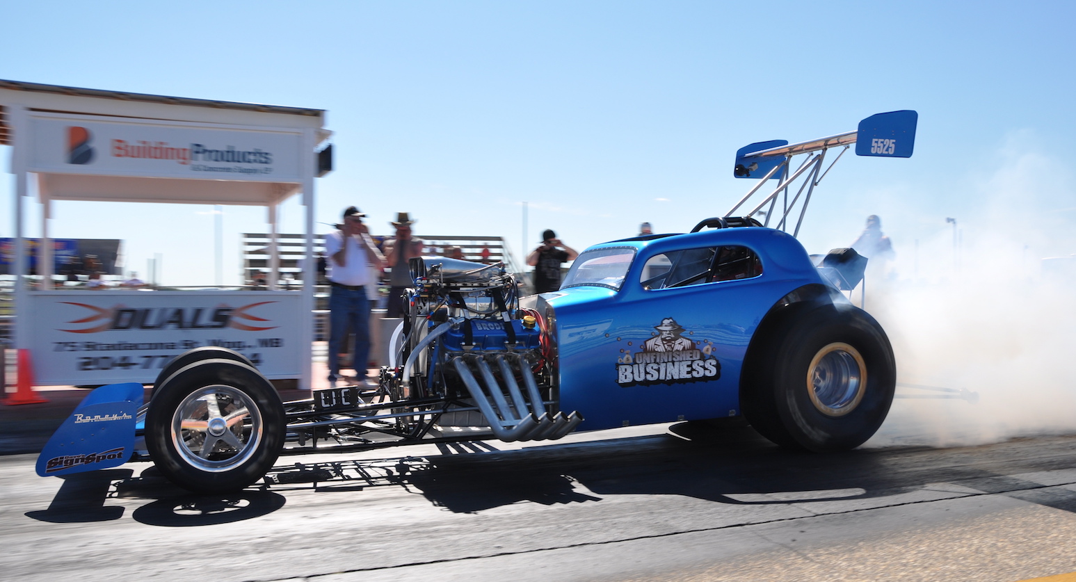
Exercise 2.8 (Drag racing)
In drag racing, specially designed cars maximize the friction with the road to achieve maximum acceleration. Consider a drag racer (or ‘dragster’) as shown in Fig. 2.8, for which the center of mass is close to the rear wheels.
Draw a free-body diagram of the dragster in side view. Draw the wheels as circles, and approximate the shape of the dragster body as a triangle with a horizontal line between the wheels, a vertical line going up from the rear axis, and a diagonal line connecting the top to the front wheels. NB: consider carefully the direction of the friction force!
On which of the wheels is the frictional force the largest?
The frictional force is maximized if the wheels just don’t slip (because, as usual, the coefficient of kinetic friction is smaller than that of static friction). Find the maximal possible frictional force on the rear wheels.
Find the maximal possible acceleration of the dragster.
For a coefficient of (static) friction of 1.0 (a fairly realistic value for rubber and concrete) and a track of 500 m, find the maximal velocity a drag racer can achieve at the end of the track when starting from rest.
Exercise 2.9 (Three blocks on a slope)
Blocks A, B and C are placed as shown in the figure, and connected by ropes of negligible mass. Both A and B weigh \(20.0\;\mathrm{N}\) each, and the coefficient of kinetic friction between each block and the surface is \(0.3\). The slope’s angle \(\theta\) equals \(42.0^\circ\). The disks in the pulleys are of negligible mass. After the blocks are released, block C descends with constant velocity.

Find the tension in the rope connecting blocks A and B.
What is the weight of block C?
If the rope connecting blocks A and B were cut, what would be the acceleration of C?
Exercise 2.10 (Seesaw)
The figure below shows a common present-day seesaw design. In addition to a beam with two seats, this seesaw also contains two identical springs that connect the beam to the ground. The distance between the pivot and each of the springs is 30.0 cm, the distance between the pivot and each of the seats is \(1.50\;\mathrm{m}\).

A 4-year-old weighing \(20.0\;\mathrm{kg}\) sits on one of the seats, causing it to drop by \(20\;\mathrm{cm}\). Draw a free-body diagram of the seesaw with the child, in which you include all relevant forces (to scale).
Use your diagram and the provided data to calculate the spring constant of the two springs present in the seesaw.
Exercise 2.11 (Two marbles in a cylindrical container)
Two marbles of identical mass \(m\) and radius \(r\) are dropped in a cylindrical container with radius \(3r\), as shown in the figure. Find the force exerted by the marbles on points A, B and C, and the force the marbles exert on each other.

Exercise 2.12 (Stacked oranges)
Round fruits like oranges and mandarins are typically stacked in alternating rows, as shown in Fig. 2.9. Suppose you have a crate with a square base that is exactly five oranges wide. You stack 25 oranges in the crate, then put another 16 on top in the holes, and then add a second layer of 25 oranges, held in place by the sides of the crate. Find the total force on the sides of the crate in this configuration. Assume all oranges are spheres with a diameter of \(8.0\;\mathrm{cm}\) and a mass of \(250\;\mathrm{g}\).

Fig. 2.9 Stacked fruit. (a) Stacked mandarins at a fruit stand [11]. (b) Cross-section of stacked oranges in a crate.#
Exercise 2.13 (Buoyancy force)
Objects with densities less than that of water float, and even objects that have higher densities are ‘lighter’ in the water. The force that’s responsible for this is known as the buoyancy force, which is equal but opposite to the gravitational force on the displaced water: \(F_\mathrm{buoyancy} = \rho_\mathrm{w} g V_\mathrm{w}\), where \(\rho_\mathrm{w}\) is the water’s density and \(V_\mathrm{w}\) the displaced volume. In parts (a) and (b), we consider a block of wood with density \(\rho < \rho_\mathrm{w}\) which is floating in water.
Which fraction of the block of wood is submerged when floating?
You push down the block somewhat more by hand, then let go. The block then oscillates on the surface of the water. Explain why, and calculate the frequency of the oscillation.
You take out the piece of wood, and now float a piece of ice in a bucket of water. On top of the ice, you place a small stone. When everything has stopped moving, you mark the water level. Then you wait till the ice has melted, and the stone has dropped to the bottom of the bucket. What has happened to the water level? Explain your answer (you can do so either qualitatively through an argument or quantitatively through a calculation).
Rubber ducks also float, but, despite the fact that they have a flat bottom, they usually do not stay upright in water. Explain why.
You drop a \(5.0\;\mathrm{kg}\) ball with a radius of \(10\;\mathrm{cm}\) and a drag coefficient \(c_d\) of \(0.20\) in water (viscosity \(1.002\;\mathrm{mPa}\cdot\mathrm{s}\)). This ball has a density higher than that of water, so it sinks. After a while, it reaches a constant velocity, known as its terminal velocity. What is the value of this terminal velocity?
When the ball in (e) has reached terminal velocity, what is the value of its Reynolds number (see Exercise 1.3)?
Exercise 2.14 (Balanced stick)
A uniform stick of mass \(M\) and length \(L = 1.00\;\mathrm{m}\) has a weight of mass \(m\) hanging from one end. The stick and the weight hang in balance on a force scale at a point \(x = 20.0\;\mathrm{cm}\) from the end of the stick. The measured force equals \(3.00\;\mathrm{N}\). Find both the mass \(M\) of the stick and \(m\) of the weight.

Exercise 2.15 (Sitting on a hinged bar)
A uniform rod with a length of 4.25 m and a mass of 47.0 kg is attached to a wall with a hinge at one end. The rod is held in horizontal position by a wire attached to its other end. The wire makes an angle of \(30.0^\circ\) with the horizontal, and is bolted to the wall directly above the hinge. If the wire can support a maximum tension of 1250 N before breaking, how far from the wall can a 75.0 kg person sit without breaking the wire?
Exercise 2.16 (A suspended bar)
A wooden bar of uniform density but varying thickness hangs suspended on two strings of negligible mass. The strings make angles \(\theta_1\) and \(\theta_2\) with the horizontal, as shown. The bar has total mass \(m\) and length \(L\). Find the distance \(x\) between the center of mass of the bar and its (thickest) end.

Exercise 2.17 (Bicycle wheel crossing a step)
A bicycle wheel of radius \(R\) and mass \(M\) is at rest against a step of height \(3R/4\), as shown in the figure. Find the minimum horizontal force \(F\) that must be applied to the axle to make the wheel start to rise over the step.

Exercise 2.18 (Force balance)
A block of mass \(M\) is pressed against a vertical wall, with a force \(F\) applied at an angle \(\theta\) with respect to the horizontal (\(-\pi/2 < \theta < \pi/2\)), as shown in the figure. The friction coefficient of the block and the wall is \(\mu\). We start with the case \(\theta=0\), i.e., the force is perpendicular to the wall.

Draw a free-body diagram showing all forces.
If the block is to remain stationary, the net force on it should be zero. Write down the equations for force balance (i.e., the sum of all forces is zero, or forces in one direction equal the forces in the opposite direction) for the x and y directions.
From the two equations you found in (b), solve for the force \(F\) needed to keep the block in place.
Now repeat the steps you took in (a)-(c) for a force under a given angle \(\theta\), and find the required force \(F\).
For what angle \(\theta\) is this minimum force \(F\) the smallest? What is the corresponding minimum value of \(F\)?
What is the limiting value of \(\theta\), below which it is not possible to keep the block up (independent of the magnitude of the force)?
Exercise 2.19 (Motion with drag)
A spherical stone of mass \(m=0.250\;\mathrm{kg}\) and radius \(R=5.0\;\mathrm{cm}\) is launched vertically from ground level with an initial speed of \(v_0=15.0\;\mathrm{m}/\mathrm{s}\). As it moves upwards, it experiences drag from the air as approximated by Stokes drag, \(F = 6 \pi \eta R v\), where the viscosity \(\eta\) of air is \(1.002\;\mathrm{mPa}\cdot\mathrm{s}\).
Which forces are acting on the stone while it moves upward?
Using Newton’s second law of motion, write down an equation of motion for the stone (this is a differential equation). Be careful with the signs. Hint: Newton’s second law of motion relates force and acceleration, and the drag force is in terms of the velocity. What is the relation between the two? Simplify the equation by introducing the characteristic time \(\tau = \frac{m}{6 \pi \eta R}\).
Find a particular solution \(v_\mathrm{p}(t)\) of your inhomogeneous differential equation from (b).
Find the solution \(v_\mathrm{h}(t)\) of the homogeneous version of your differential equation.
Use the results from (c) and (d) and the initial condition to find the general solution \(v(t)\) of your differential equation.
From (e), find the time at which the stone reaches its maximum height.
From \(v(t)\), find \(h(t)\) for the stone (height as a function of time).
Using your answers to (f) and (g), find the maximum height the stone reaches.