
10.4. Exercises#
Each exercise carries the difficulty level indication:
[*] Easy
[**] Moderate
[***] Advanced
🖌️ Uses the NaNoPy graphical environment
The highest difficulty level is meant for students who wish to challenge themselves and/or have previous experience in programming.
Important
Do all NaNoPy exercises (🖌️), whatever their difficulty level. They build on each other, so skipping one makes the next ones harder.
Exercise 10.8 ([*] Basics of NumPy)
This exercise contains a number of simple things to try to get familiar with NumPy.
Hint: Functions (probably) exist for most of these.
Use the NumPy documentation at numpy.org - try not to be too intimidated, it’s easier than it seems.
Google is also your friend.
import numpy as np
Exercise A
Define x_ar so that it is an array of 124 elements ranging from 2.3 to
1776.343, evenly spaced on a logarithmic scale.
Hint: There is a function to do this.
x_ar = # Your code here
Exercise B
Reshape x_ar to 2-dimensional array (pick the lengths you’d like).
# Your code here
Exercise C
Add 10 to every value in the array.
Hint: you don’t need any loops to do so.
# Your code here
Exercise D
Reshape x_ar to a 1-dimensional array again.
Define a new array y_ar as a linear space of 10 values from 23.4 to 1006.2
and add it to the end of x_ar.
# Your code here
Exercise E
Print every 10th value from the new combined x_ar. You should be able to do
this without loops.
# Your code here
Exercise F
Test out this code. Try to describe what you see and understand what is going on before running it).
test_ar = np.linspace(1, 50)
mask_ar = test_ar >= 25
new_ar = test_ar[mask_ar]
print(new_ar)
Exercise G
Now find the average for every value above 100 in the combined x_ar.
You should be able to do this without loops.
# Your code here
Exercise 10.9 ([*] How many ways to the same array?)
How many ways to the same array?
In each of the exercises below, you will receive an array. There is typically more than one way to define an array in NumPy. Therefore, for each of the arrays below, try to think of at least two (and if possible more) ways to define them using NumPy’s functions and write the corresponding Python code. If you feel like it, you can also make it into a competition with your fellow students, or a competition between student groups! Feel free to use NumPy documentation.
Exercise A:
A = [ 0 1 2 3 4 5 6 7 8 9 10 ]
Exercise B:
B = [ 1 1 1 1 1 1 ]
Exercise C:
C = [ 0 0 0 0 ] [ 0 0 0 0 ]
Exercise D:
D = [ 2 0 0 ] [ 0 2 0 ] [ 0 0 2 ]
Exercise E:
E = [ 5 0 0 ] [ 5 5 0 ] [ 5 5 5 ]
Exercise F:
F = [ 1 1 1 ] [ 1 1 1 ] [ 1 1 1 ]
Exercise G:
G = [ 2 4 6 8 10 12 14 16 18 20 ]
Exercise H:
H = [ 1 0 0 0 ] [ 0 5 0 0 ] [ 0 0 -9 0 ] [ 0 0 0 -2 ]
Exercise 10.10 ([*] List with the highest mean)
Find the list which has the highest mean and the value of that mean. Inform the user about your findings using print statements.
Start with writing pseudocode.
Hints:
Which NumPy function could come handy here?
Use a for loop and track the highest mean
list1 = [3, 5, 7, 9, 2, 4, 6, 8, 10, 1, 3, 5]
list2 = [7, 9, 2, 4, 7, 5, 3, 1, 8, 6]
list3 = [2, 4, 6, 9, 10, 3, 5, 6, 9]
list4 = [1, 3, 5, 7, 9, 1, 3, 5, 7, 2, 4, 6, 8, 10]
list5 = [4, 6, 8, 10, 2, 4, 6, 8, 10, 1, 3, 5, 7, 9]

# Your code here
Exercise 10.11 ([*] Drawing parametric curves 🖌️)
Parametric equations relate a control parameter t to functions x(t) and y(t). Plotting x(t) and y(t) for a range of t can produce some funky curves.
(A) Create a NaNoPy Canvas of size 100 by 100.
(B) Use NumPy’s linspace(...) function to define a range of values of t from
-10 to 10.
(C) Calculate the values of x and y produced by the equations
x(t) = 10 sin(t) + 40
y(t) = t^2
(D) Draw every pair of (x(t), y(t)) onto your canvas using the pen’s
draw_pixel(...) function.
(E) Look for other funky parametric curves online.
Exercise 10.12 ([**] Kinetic energy)
Kinetic energy
Given a NumPy array of masses, calculate the kinetic energy of objects using E = 1/2 m*v^2, where m is mass and v = 10 nm/s is velocity.
Use these masses (given in micrograms): [1.5, 2.0, 2.5, 3.0, 3.5, 50, 100].
# Your code here
Exercise 10.13 ([**] Bacterial growth)
A bacterial population grows exponentially according to this equation: N(t) = N_0 * e^(rt), where N(t) is number of bacteria in time t, N_0 is initial number of bacteria, r is growth rate, and t is time.
Exercise A: Population size
Given N_0 = 1,000 and r = 0.2 per hour, calculate bacterial population size every hour for time ranging from 0 to 48 hours. Use NumPy arrays.
# Your code here
Exercise B: Induction of protein expression
In the lab, you’re growing a culture of 100 mL of Escherichia coli that you transformed with a plasmid containing your favourite protein-coding gene. The initial number of cells is 2 * 10^6. You want to grow E. coli until the culture reaches an optical density (OD_600) of 0.6. This value indicates an exponential growth phase and is optimal time for induction of protein expression.
Knowing that for E. coli 1 OD_600 = 5 * 10^8 cells/mL and that it grows with a rate of 0.3 per hour, calculate how much time you need to grow E. coli before induction.
# Your code here
Exercise 10.14 ([**] Protein concentration)
A biologist has measured the concentration of their favourite protein in cell lysates over time, recorded in 10-minute intervals over a 24-hour period. The concentrations are stored in a 1D NumPy array.
import numpy as np

np.random.seed(0) # Setting seed for random number generation for reproducibility
time_points = np.arange(0, 1440, 10) # Time in minutes
protein_concentration = np.random.uniform(0.1, 1.0, len(time_points)) # Concentrations in nmol/L
Exercise A: Extract the concentrations between the 6th and 10th hours and print them.
# Your code here
Exercise B: Get concentrations measured at every full hour and print them.
# Your code here
Exercise C: Extract the concentrations from the last 3 hours and print them.
# Your code here
Exercise 10.15 ([**] Heat distribution in a metal plate)
A 9x9 grid represents a metal plate where each cell indicates the temperature at that point. The temperature is stored in a 2D NumPy array.
import numpy as np

# Heat distribution across a 9x9 metal plate
np.random.seed(0) # Setting seed for random number generation for reproducibility
heat_distribution = np.random.uniform(20, 100, (9, 9)) # Degrees Celsius
Exercise A: Extract the temperatures from the top-left 3x3 corner of the plate.
# Your code here
Exercise B: Extract the middle row and the middle column and print them.
# Your code here
Exercise C: Get the temperatures along the diagonal of the plate and print them.
# Your code here
Exercise D: You can imagine your 9x9 plate consisting of 9 3x3 subplates (similar to when you’re solving Sudoku puzzles). Calculate which of the 9 3x3 subplates has the highest average temperature and print the result.
# Your code here
Exercise 10.16 ([**] Social network for epidemic modelling)
Social network
As you might imagine from the experience of the recent years, modelling an epidemic spread is rather useful. One of the possible models is the so-called “probabilistic network model”, in which we model pathogen spread in the group via a network of social contacts. As it turns out, a social network can conveniently be represented by a matrix W. Let’s look at an example:
W = [ 1 1 0 ] [ 1 1 1 ] [ 0 1 1 ]
You can imagine each row and each column representing a person. Our example matrix W therefore outlines a social network of 3 people. When two individuals know each other, the corresponding element in the matrix is 1. In matrix terminology, we can say that element w_ij = 1 when persons i and j know each other. The matrix is also symmetrical, i.e., w_ij = w_ji. If w_ii = 1, then i abides by Socrate’s advice: “know thyself”.
Remember: in w_ij, i denotes the row and j the column.
Below we give you a social network matrix W to use in the exercises. We also offer some general tips/hints to keep in mind:
Matrix is symmetric, so (when applicable) make sure not to count the same contact twice.
When looking at contacts between differet individuals, you can exclude elements from matrix diagonal (i.e., the “know thyself” elements).
Remember good coding practices and avoid hardcoding. Your code should work for any social network matrix.
import numpy as np

# Define social network matrix
num_people = 20 # Matrix of 20 people
np.random.seed(0) # Setting seed for random number generation for reproducibility
W = np.random.choice([0, 1], size=(num_people, num_people), p=[0.6, 0.4]) # Matrix with random 0s and 1s, 0 appears with 60% probability
W = np.tril(W) + np.transpose(np.tril(W)) # Making the matrix symmetric by using the lower triangular part and its transpose
np.fill_diagonal(W, 1) # Set diagonal elements to 1
Exercise A: Person number 5
How many contacts does person number 5 have? Use Python to find the answer and print it.
Hint: How does counting in Python work?
# Your code here
Exercise B: The influencer
Find out which person in your social network has the most contacts (i.e., who’s the influencer)? Make a print statement about it.
# Your code here
Exercise C: Interconnectedness
How many social contacts in total are represented in W? Calculate and make a print statement.
# Your code here
Exercise D: A new friendship
Two people have met at a party, so now they also know each other. Make a new social network matrix W_new that also contains this contact. In practice, identify two people in your matrix W that have not known each other (w_ij = 0) and turn the corresponding matrix element(s) to 1.
Is the influecer still the same person? You can reuse your code from above to find out.
# Your code here
Exercise 10.17 ([**] Dataset Manipulation)
You are doing an experiment that requires you to measure voltages at different timepoints. After your measurements are done, you are left with the following dataset. To this set of voltages, you are asked to apply a number of operations in order to retrieve some information from it.
Note that some tasks can be done with the tools that you have learnt but might be easier using other built-in functions. After writing your own code for those you are able to, compare your own answer to that given by AI.
A: Clip the data, such that all values above 100 and below 0 are discarded
B: Find the number of unique values that occur in the array
C: Calculate the cumulative total value at each step
D: Determine the change of the signal for each measurement
E: Shift the entire signal forward by three steps, wrapping around
F: Find the positions of all values equal to 60
G: Determine the range (maximum and minimum value) of the cleaned signal
import numpy as np

sensor_data = np.array([102, 98, 95, 93, 500, 7, 6, 92, 91, 89, 88, 87, -40, -45, -50, 233, 86, 85, 84, 70, 93, 59, 7, 33, 88, 87, 9, 60, 9, 8, 5, -2, -8, -10, -12, -15, 60, 59, 58, 10, -20, -25, -30, -35])

# Your code here
Exercise 10.18 ([**] Drawing arrays 🖌️)
NaNoPy can be used for rudimentary plotting, but you have to build the tools yourself. Later in the book, more effective methods for plotting will be introduced.
This exercise is also intended as practice for deciphering code written by other authors. While exploring the code below, place comments describing what is happening.
import numpy as np
from NaNoPy import Writer, Canvas, Color

x = np.linspace(-3, 3, 80)
y = np.linspace(1.5, -1.5, 40).reshape(40, 1)
value = x**2 + y**2 + x * y
image_1 = (127.5 + 127.5 * np.sin(value.reshape(40, 80, 1) + np.array([0, 2, 4]))).astype(np.uint8)

x_2 = np.linspace(-2.2, 0.8, 80)
y_2 = np.linspace(1.2, -1.2, 40).reshape(40, 1)
c = x_2 + 1j * y_2
z = np.zeros_like(c)
steps = np.zeros_like(c)
for i in range(30):
    z = np.where(np.abs(z) < 2, z**2 + c, z)
    steps = steps + np.abs(z)

image_2_monochrome = steps.reshape(40, 80, 1) * np.array([0, 1, 2])
image_2 = image_2_monochrome.astype(np.uint8)
Problem 1
(A) What does .reshape(40,1) do to y? What shapes do the arrays x, y,
and x + y have?
(B) Decipher the operations performed to create image_1 and image_2. Draw a
matching flowchart on paper for each.
(C) What does .astype(np.uint8) do? Google it or ask an LLM.
# Collapse me in VS Code
image_3 = np.array([
    ...
], dtype=np.uint8).reshape(40, 80, 3)
Problem 2 Each of the arrays contains the RGB values of an image per pixel.
(A) Draw one of the images above to a NaNoPy canvas using Writer.draw_pixel().
Hint: You can create custom colors using NaNoPy’s Color.custom(r=..., g=..., b=...)
(B) Update the screen after every ten pixels drawn to animate the image.
The RGB colors “live” in the cube between (0, 0, 0) and (255, 255, 255). You can transform one color into another color using vectorized operations.
(C) Reduce the brightness of the image by a factor 2.
The operation: image[:, :, [2, 0, 1]] switches the order of the color channels.
Since this does not change the shape of the array, you can interpolate between
the original image and the modified image.
(D) Animate the image by interpolating between the images with different weights.
Hint: Color.custom(...) does not accept values above 255. You can use NumPy’s
clip() function to avoid this issue.
Exercise 10.19 ([**] Predator vs. prey 🖌️)
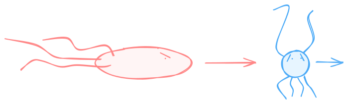
There exist predator-prey relationships among microorganisms. Both predator and prey can evolve sophisticated methods for hunting and evading respectively. This exercise is designed to have you simulate a simplified version of such behaviour:
A predator always moves in the direction of the closest prey
A prey always moves away from the closest predator
Try to use the vectorization capability of NumPy as much as possible in the following problems, only using for-loops to keep track of time.
import numpy as np
from NaNoPy import Canvas, Writer, Color

screen = Canvas("Predator vs. Prey", x_size=1000, y_size=1000)
pen = Writer(screen)


predator = np.array([50., 50.])
prey = np.array([100., 100.])
Problem 1: One predator vs. one prey microbe
predator and prey each contain xy-coordinates.
(A) Draw a red circle for the predator and a blue circle for the prey with NaNoPy.
(B) Calculate the Euclidean distance between predator and prey.
(C) Calculate the unit-direction from predator to prey.
Hint: This is the difference between their positions normalized by the distance.
(D) Move both predator and prey in this direction with speeds 2 / frame and 1 / frame respectively.
(E) Repeat this cycle using a for-loop.
(F) Stop the loop if the distance between predator and prey is smaller than one.
# your code here!
Problem 2: Many predators vs. one prey microbe
Adding multiple predators means that you need to find the closest predator from the prey’s perspective to decide how it moves.
(A) Create an array predators of shape (n_predators, 2) to store the positions
of all predators.
(B) Adapt the drawing logic to draw all predators.
(C) Calculate the Euclidean distance between the prey and every predator, as an
array of shape (n_predators,). This requires taking a sum. Use the
axis=... keyword to specify which part of the array the sum should be
taken over.
(D) Find the closest predator from the perspective of the prey.
(E) Calculate the direction for each predator (remember to vectorize!)
(F) Adapt the code for updating the positions to accommodate multiple predators.
# your code here!
Bonus problem (ADVANCED): Many predators vs. many prey microbes
Solving this problem using only vectorization is quite tricky. You will not be provided with detailed instructions, but here are some hints:
You can represent a pair of coordinates (x, y) as a complex number x + i y. This makes it easier to have every predator interact with every prey.
positions = x_array + 1j * y_array
x_array = positions.real
y_array = positions.imag
One advantage of this approach is that it makes it very simple to calculate the distance between two positions:
distance = np.abs(pos_2 - pos_1)
A_grid, B_grid = np.meshgrid(A, B)produces a grid of A-values and a grid of B-values where every element ofAis aligned with every element ofBexactly once. A_grid and B_grid have the same shape, which makes it nice to combine them in vectorized operations.You need to find the closest predator for each prey and the closest prey for each predator. They are not necessarily the same. This also means that you have to keep track of a direction for each prey and a direction for each predator.
You can “spice up” the problem by removing caught prey. Doing this without changing the size of the array (pure vectorization) requires masking with another array.