1. The emergence of quantum mechanics

1.1. Historical context: experiments that contradict the predictions of classical physics

Special relativity came about because people couldn’t find something they thought was there: the ether filling all of space, providing the medium for electromagnetic waves to propagate in. If there was no ether, such waves, and specifically light, had to be able to propagate in vacuum. Moreover, and much more unsettling, no ether meant that the very axioms on which physics was based were wrong. There is no instantaneous action at a distance, and accelerations are not absolute. A new set of axioms was required, provided by Einstein in his two postulates: that of relativity, and that of the universality of the speed of light [Idema, 2018].

Not being able to find the ether wasn’t the only problem physicists at the end of the 19th century faced. There were a few more nagging issues that seemed, at the time, to be rather minor, but yet unresolved.

1.1.1. The ultraviolet catastrophe

One problem people had trouble explaining was the emission spectrum of a black body. Black bodies are objects that absorb all incoming electromagnetic radiation, irrespective of frequency or the angle of incidence (you can guess why they’re called black). Electromagnetic radiation carries energy, and by absorbing it, the black body heats up. If the black body becomes warmer than its environment, by the laws of thermodynamics, it will release some of the heat again, also in the form of electromagnetic radiation. However, for a black body, the emitted radiation has no relation to the absorbed radiation. Emission happens in a wide range of frequencies, and depends only on the temperature of the black body. The amount of radiation in each frequency (or equivalently, at each wavelength^[1]) is what we refer to as the black body’s emission spectrum. Emission spectra for black bodies at various temperatures are shown in Fig. 1.1. The best available classical model for the emission spectrum was the Rayleigh-Jeans law, which gives a reasonable approximation at low frequency / long wavelength. However, it fails dramatically at higher frequencies, or towards the (ultra)violet part of the electromagnetic spectrum, where it incorrectly predicts that the emission intensity keeps increasing with frequency - hence the name ‘ultraviolet catastrophe’.

Fig. 1.1 Emission spectrum of a black body at temperatures of \(3000\;\mathrm{K}\), \(4000\;\mathrm{K}\) and \(5000\;\mathrm{K}\), as a function of the emission wavelength. Note that the peak of the spectrum at \(5000\;\mathrm{K}\) overlaps with the range of visible light. The black dashed line shows the classical result (Rayleigh-Jeans law) at \(5000\;\mathrm{K}\), illustrating its dramatic failure at short wavelengths (known as the ultraviolet catastrophe). Image adopted from ^[2].

1.1.2. The photo-electric effect

Another strange phenomenon that cannot be explained with classical physics is the onset of what is known as the photo-electric effect. If you shine a light beam of sufficient intensity on a piece of metal, the metal will absorb the light and emit electrons, easily measurable as a current through the metal. So far no problem: obviously some of the energy in the light is transferred to electrons in the metal, which become free electrons and start a current. It is also hardly surprising that the resulting current depends on the intensity of the light. However, what was completely unexplainable was that whether or not the effect occurred at all depended on the frequency of the light. Every metal has its own critical frequency. If you shine light of a lower frequency on it, no matter how intense your beam is, you will not get a current.

1.1.3. The stability of atoms

Around the start of the twentieth century, experimentalists (notably Rutherford, but also many others) had made great progress in revealing the structure of atoms. People knew they had a nucleus in which the positive charge was located, that the type of atom was determined by the number of protons (equal to the number of elementary positive charges) in the nucleus, and that the nucleus was surrounded by orbiting electrons - as many as there are protons for a neutral atom (see Fig. 1.3a). A shell model for the atom explained a lot of chemistry. In this picture, there are a number of shells around the nucleus in which an electron can exist, with the lowest (known as the K shell) capable of holding two atoms, the next (L and M shell) eight each, the next two eighteen, and so on. Atoms would have a tendency to fill their outer shell, bonding with other atoms and sharing electrons where necessary, so hydrogen needs one electron, oxygen two, carbon four, and helium none. The vacancies in the outer shell then explain why you can have molecular hydrogen (\(\mathrm{H}_2\)), water (\(\mathrm{H}_2\mathrm{O}\)), methane (\(\mathrm{C}\mathrm{H}_4\)), and carbon dioxide (\(\mathrm{C}\mathrm{O}_2\)), each oxygen sharing two electrons with the carbon, and a helium atom would be a molecule all by itself (\(\mathrm{He}\)). The problem, however, was that according to classical mechanics, the orbits of the electrons around the nucleus would be unstable - an orbit closer to the nucleus corresponds to a lower energy state, and thus the orbits would spontaneously decay, releasing energy by the emission of electromagnetic radiation, much like the black body. Classically, there is nothing stopping the electron from dissipating all of its orbital energy in that way - which means that it should rapidly crash into the nucleus. Obviously, and fortunately for us, that is not the case.

1.2. Quantization

1.2.1. Light: quantization of energy

As it turns out, all three puzzles in the previous section can be solved if you make one specific assumption, but one so counter-intuitive that it took people a long time to take it seriously. The essence of the assumption is that energy is not a continuous quantity, as assumed in classical physics, but a discrete one. We say that energy is quantized, that is, there is a smallest possible amount of energy (a quantum), which cannot be divided into smaller parts.

The first person to use this idea was Max Planck, in an attempt to solve the puzzle of the ultraviolet catastrophe. Quantizing the energy of the radiation as it is emitted by a black body, Planck was able to derive an equation for the emission spectrum that fits the data beautifully. However, although Planck assumed that the emitted radiation came in discrete packages, he did not push this idea to the next step: that the energy in any kind of electromagnetic radiation is quantized. That assumption was made by Einstein, in an attempt to solve the second puzzle. Einstein postulated that the energy of electromagnetic radiation is always quantized, and that the amount of energy in a quantum depends on the frequency^[3]. He introduced the idea of the energy quantum, carrying an amount of energy given by \(E_\mathrm{quantum} = h \nu\), where \(\nu\) is the frequency and \(h\) is a physical constant known today as Planck’s constant. We call Einstein’s quanta of electromagnetic radiation photons. The existence of photons was initially widely disputed, but the solution of the photo-electric effect puzzle eventually earned Einstein his Nobel prize.

Once you assume that Einstein was right about the photons, understanding the photo-electric effect is pretty straightforward. The atoms in a metal contain a few electrons which are only weakly bound to their nucleus by electromagnetic forces. It is therefore easy to peal such an electron off its atom, creating a free negatively charged electron (leaving a positively charged ion), which can then move through the metal; that is why metals conduct electricity. However, even though creating a free electron is relatively easy, it still requires a certain amount of energy. In the case of the photo-electric effect, that energy is provided by the incident light. If we accept that the energy in that light is quantized, it follows that a quantum of energy (or photon, as we’ll refer to them from now on) must be large enough to provide the energy needed to free an electron for the effect to occur at all. For low-frequency light, by Einstein’s second assumption, the energy of a photon is small. For some metals, the photon’s energy will be too small to free any electron. Therefore, for those metals, no current is found. Increasing the intensity of the light beam increases the amount of photons, not the energy per photon^[4]. For higher-frequency light the photons carry more energy, and will therefore be able to free electrons by transferring that energy to them. Now more photons means more free electrons, so a higher current.

All this may seem perfectly reasonable to you, but if so, take a step back and think about what we’ve just done: we’ve described light as a stream of particles. We know that to be wrong. Light is a wave, as is easily verified by the fact that it exhibits interference, which would be very odd for particles. To illustrate this point, let us go back in time^[5] to the experiment that actually showed that light is a wave: Young’s double-slit experiment (see Fig. 1.2). In Young’s setup, light is shone on a board with two slits in it, and the resulting pattern visualized on a screen behind the board. What you see is an interference pattern: alternating stripes of low and high intensity light. This pattern can easily be understood from the wave nature of light: the two slits act as sources, emitting waves of the same frequency and phase, which interfere sometimes constructively (giving high-intensity stripes) and sometimes destructively (giving low-intensity stripes), Fig. 1.2b. Now imagine doing the same experiment with particles. There is no way you will get interference. Most particles will be stopped by the board, some will pass through the slits and hit the screen. If multiple particles hit at the same spot, the intensity of the spot will increase; intensity will be low where few particles hit. You’ll get a completely different pattern, as shown in Fig. 1.2c.

Fig. 1.2 Schematic depiction of Young’s double slit experiment. (a) Setup. (b) Interference pattern for waves. (c) Intensity pattern for (classical) particles.

Now we have a problem. Young’s experiment shows light to be a wave, while the photo-electric effect can only be explained by assuming light exists of a stream of discrete particles. This is not a paradox, it’s a real contradiction. In classical physics, it has to be either one, not both.

Unfortunately, there is no neat way out. In some experiments light behaves as a wave, in some as a particle. Light thus must have aspects of both, even if that is contradictory in the classical sense. In quantum mechanics, we accept this contradiction as an axiom, and say that light has both a particle and a wave nature. The two are coupled through Einstein’s relation for the energy of the photon, \(E_\mathrm{photon} = h \nu\), which relates a particle property, its energy, to a wave property, its frequency. Nobody knows or understands why this is the case. We only know that our experiments tell us that it has to be true.

1.2.2. Matter: quantization of (angular) momentum

If energy is quantized (once again, this means that there exists a smallest, undividable quantum of energy), we could ask the question if the same can be true for other physical quantities, like momentum and angular momentum. To solve the third puzzle, we need to do exactly that. In 1923, Niels Bohr developed a model for the hydrogen atom, based on the assumption that the angular momentum of the single electron orbiting the one-proton nucleus was quantized, and found that his model could predict the emission spectrum of hydrogen, which consists of a collection of very sharply defined frequencies and nothing in between. We’ll look at that model from a slightly different point of view, based on an observation by Louis de Broglie that came two years later. De Broglie’s idea was that if light, which we know as a wave, can exhibit particle-like behavior, maybe objects we know as particles, such as electrons, could exhibit wave-like behavior as well. De Broglie postulated that Einstein’s relation between the energy and frequency of a photon might hold for any particle. Second, De Broglie postulated that, since energy and momentum are related, momentum must be related to a wave property as well. We then have, for any particle / wave:

(1.1)\[\begin{align*} E &= h \nu = \hbar \omega,\ \end{align*}\]

(1.2)\[\begin{align*} p &= h / \lambda = \hbar k. \end{align*}\]

Here \(\nu\) is the frequency, \(\lambda\) the wavelength, \(\omega = 2\pi\nu\) the angular frequency, \(k = 2\pi / \lambda\) the (angular) wavenumber, and \(\hbar = h / 2\pi\). As before, we have \(v = \lambda \nu = \omega / k\) for the speed of the wave. Note that equations (1.1) and (1.2) also allow us to define the momentum of a photon, by \(p = \hbar k = \hbar \omega / c = E / c\), with \(c\) the speed of light^[6]. The energy in (1.1) is the particle’s total energy, including the rest energy of special relativity, \(E=mc^2\).

Before we go into the Bohr model, a sensible question to ask is if there is any experimental evidence for the De Broglie hypothesis. We’ve seen that for light, the explanation of some experiments requires a wave model while others require a particle model. We know electrons (for instance) behave like particles in classical experiments, and it does seem reasonable to expect that if we put them in a Young’s double-slit type experiment, we would observe something like Fig. 1.2c. We do, but only if the slits are as wide as in a typical light experiment. However, if we make them smaller, electrons start exhibiting interference patterns as well, even if we release them one at the time. This effect is at least as absurd as taking a wave phenomenon like light to be quantized. It means that every single electron interferes with itself. In quantum mechanics, rather than saying that the electron takes the left or the right slit, as we would classically, we say that there is a probability that it takes the right slit, and a (potentially different) probability it takes the left one. The two possible realizations then interfere with each other as if they were waves, indeed creating an interference pattern. We’ll return to this idea of probabilities in the next section.

The reason why people in Young’s time did not see interference patterns in particle streams is simple: their wavelength is much shorter than that of light. A photon from the visible spectrum has a wavelength between roughly \(300\) and \(800\;\mathrm{nm}\); to get an interference pattern, the width of the slits needs to be in the same range, though slightly bigger still works. The typical wavelength of an electron is about a tenth of a nanometer, a thousand times smaller than that of light. For electrons, Young’s slits aren’t slits at all, but very wide openings, which is why they don’t exhibit interference in Young’s original setup.

Now, assuming de Broglie was right and things we always thought of as particles can behave like waves, can we understand the stability of the atom? Let us consider the simplest case, hydrogen, where one negatively charged electron orbits a positively charged nucleus consisting of one proton. Since the proton is much heavier than the electron, we’ll assume it is stationary. If the electron is a wave, the length of its orbit must correspond to an integer number of wavelengths: it has to close on itself, giving similar restrictions as waves in guitar strings and organ pipes. Say the radius of the orbit is \(r\), then \(2 \pi r = n \lambda\), where \(n\) is some integer. Other orbits than these, i.e., orbits of which the circumference is not an integer multiple of the electron’s wavelength, are not allowed. This approach is again very different from the classical picture. There is no reason to deny a particle any specific orbit. For waves, on the other hand, there is no reason to assume anything but discrete orbits, just like you can only produce a discrete set of frequencies with a given guitar string.

Fig. 1.3 Two models of the atom. (a) Classical Rutherford model with the electrons in fixed orbits around the nucleus. (b) Bohr model. Negatively charged electrons (charge -e) orbit the positively charged nucleus (charge \(+Ze\)) only in specific orbits, corresponding to quantized values of the angular momentum. Consequently, also the possible energy levels are quantized. Other orbits are forbidden, but electrons can ‘jump’ from a higher orbit to a lower one by emitting a photon which carries off the extra energy; they can also be induced to jump to a higher orbit by absorbing a photon with exactly the right energy.

Continuing with De Broglie’s rule for momentum (1.2), we have \(p = h / \lambda = h n / 2 \pi r\), so the momentum of the electron is quantized. The same goes for the angular momentum, which is given by \(L = p r = h n / 2 \pi = \hbar n\) (Bohr originally simply assumed this expression for the quantization of the angular momentum, just like Einstein assumed his equation for the quantization of energy, and worked from there). Taking the opposite view, of the electron as a particle, we can also calculate its (angular) momentum. The electron is kept in its circular orbit by a Coulomb force, and because it exhibits circular motion, the net force is the centripetal force, so we can write down a force balance:

(1.3)\[ \frac{1}{4 \pi \varepsilon_0}\frac{e^2}{r^2} = \frac{m_\mathrm{e} v^2}{r}, \]

from which we can calculate the electron’s speed:

(1.4)\[ v = \sqrt{\frac{e^2}{4 \pi \varepsilon_0 m_\mathrm{e} r}}. \]

Using (1.4) to calculate the angular momentum, and the quantized expression \(L = \hbar n\) found above, we arrive at an expression for the allowed orbital radii

(1.5)\[ r_n = \frac{4 \pi \varepsilon_0 \hbar^2}{e^2 m_\mathrm{e}} n^2 = a n^2, \]

where \(m_\mathrm{e}\) is the electron mass. The smallest possible value of \(r_n\) at \(n=1\) is called the Bohr radius \(a\), which is approximately equal to \(5.3 \cdot 10^{-11} \;\mathrm{m}\).

We can also calculate the electron’s energy

(1.6)\[ E = \frac12 m_\mathrm{e} v^2 - \frac{e^2}{4 \pi \varepsilon_0 r} = - \frac{e^2}{8 \pi \varepsilon_0 r} = - \frac{e^4 m_\mathrm{e}}{2(4 \pi \varepsilon_0 \hbar)^2 n^2} = - \frac{R_\mathrm{E}}{n^2}, \]

where \(R_\mathrm{E}\) is the Rydberg energy, given by

(1.7)\[ R_\mathrm{E} = \frac{e^2}{8 \pi \varepsilon_0 a} = \frac{e^4 m_\mathrm{e}}{2(4 \pi \varepsilon_0 \hbar)^2} = \frac12 (m_\mathrm{e} c^2) \alpha^2 \approx 13.6 \;\mathrm{eV}. \]

In equation (1.7), we recognize \(m_\mathrm{e} c^2\) as the electron’s rest energy from special relativity, and a new constant \(\alpha\), known as the fine structure constant, which has a numerical value very close to \(1/137\). All of these constants will return in our more detailed study of quantum phenomena in the following chapters.

Summarizing, we find that the electron in a hydrogen atom can exist in a discrete set of stable orbits with radii given by equation (1.5) and associated energies given by (1.6). ‘Higher’ orbits with larger radii carry more energy. An electron in the lowest possible orbit will thus be globally stable. If this were classical physics, the higher orbits would not be globally stable (since there are orbits with lower energy), but there would be no way to transition between orbits, as no intermediate options exist. Again, we have arrived at a point where quantum physics is completely different, because electrons actually can, and do, transition to lower orbits. They do so by emitting a quantum of energy that equals the difference in energy between the two orbits. This quantum of energy is nothing but a piece of electromagnetic radiation, i.e., a photon, with a frequency given by Einstein’s relation \(E = h \nu\). Inversely, an electron in a lower orbit can also transition to a higher orbit by absorbing a photon with exactly the right energy. We thus arrive at a testable prediction: if we observe a hydrogen atom in an excited state (meaning that the electron is in a higher orbit), we expect it to spontaneously emit light of a very specific frequency, or rather a number of specific frequencies, corresponding to the possible transitions. On the other hand, if we shine a continuous spectrum of light on an atom in the ground state (with the electron in the lowest-energy orbit), we expect it to absorb light at those frequencies. Both of these expectations exactly match experimental observations. A number of possible emission frequencies is shown in Fig. 1.4. We use them nowadays in lasers and streetlights. Absorption spectra are extensively used in astronomy: by measuring the emission from a star, and determining which frequencies are missing (because they are absorbed by atoms in the atmosphere of the star, or even more exciting, exoplanets moving in front of the star), you can determine which gasses are present in the atmosphere of that star or planet. With this method, helium was originally discovered by analyzing the atmosphere of the sun.

Bohr mixed classical and quantum physics to arrive at his hydrogen model. He used quantum ideas for discretizing energies, momenta and radii, and classical ones for the electrostatic interaction between electron and proton. The Bohr model works fairly well for hydrogen, but not so well for more complicated atoms, even the next simplest one, helium (with two electrons and a nucleus with two protons and two neutrons). However, it works quite nicely for heavier atoms if they are ionized to the point that they have only one electron left. The only thing that changes is that the nuclear charge becomes \(Ze\), with \(Z\) the number of protons. For a complete quantum description, we need a quantum set of axioms. One of those is given by De Broglie’s relations, but those are not sufficient; we’ll also need an equivalent of Newton’s second law of motion. Before we can go there, things are going to turn even weirder than they already are.

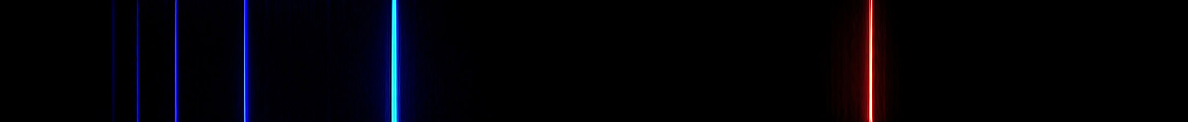
Fig. 1.4 Visible part of the emission spectrum for the Bohr hydrogen atom ^[7]. The visible lines are from the Balmer series, which are transitions from states with \(n \geq 3\) to \(n=2\). The four visible spectrum wavelengths are \(656\), \(486\), \(434\) and \(410\;\mathrm{nm}\); also visible (but technically ultraviolet) are two lines at \(397\) and \(389\;\mathrm{nm}\).

1.3. A probabilistic picture of the world

In classical physics, some processes happen spontaneously, while others require the input of energy. In a friction- and dissipation-free classical mechanics setting (accurate for e.g. the motion of planets through space), the energy of a system is conserved, which gives us stable planetary orbits around the sun. Once friction comes into play, energy can spontaneously decrease, but never increase, and so water will flow down to the ocean, but needs energy from the sun to evaporate and be deposited again on a mountain in the form of rain or snow. All these processes are deterministic: if you know the initial condition, you can (in principle) calculate what will happen at any future point in time.

Quantum particles are fundamentally different from classical ones in three ways. Two of these we already encountered: they have a dual particle-wave nature, and their properties (such as energy or angular momentum) may be quantized^[8]. The third difference is that quantum theory is not deterministic but stochastic: even if you know exactly where a particle is at a given point in time, all you can calculate is the probability of it being at a certain place at a later point in time. Consequently, even if you set up (or ‘prepare’) two systems in exactly the same physical state, and let them evolve over time, a later measurement of a physical property (an ‘observable’, such as position, momentum, or energy) of the two systems may give you different results. These differences are not measurement errors^[9], but fundamental to the quantum world.

We do not know why quantum particles behave in a probabilistic manner, but experiments have proven beyond doubt that they do. Quantum particles have a finite chance to ‘roll uphill’, jump over energy barriers (or between discrete orbital states), or interfere with themselves (as we’ve seen in the double-slit experiment with electrons). We’ll encounter specific predictions and tests of these predictions in later sections. For now, we need a new way to describe our particles, as the classical way, specifying the position as a function of time, or \(x(t)\), no longer suffices. Instead, we introduce a new object, commonly known as the wave function \(\Psi(x, t)\), which contains all information about our particle. The square of this wave function gives us the probability of finding the particle at a certain place at a given time.

1.3.1. Wave function and particle probability density

The interpretation of the wave function is one of the axioms of quantum mechanics.

Axiom 1.1 (Statistical interpretation of the wave function)

For a particle described by the wave function \(\Psi(x, t)\), the probability of finding the particle in the interval \((x, x+\mathrm{d}x)\) at time \(t\) is given by

(1.8)\[ P\big(\text{particle in }(x, x+\mathrm{d}x)\big) = \left|\Psi(x,t)\right|^2 \mathrm{d}x. \]

The probability of finding the particle in any larger interval (say between \(x_1\) and \(x_2\)) is then the sum of the probabilities for each of the infinitesimal intervals of length \(\mathrm{d}x\) that make up this larger interval, in other words, the integral:

(1.9)\[ P\big(\text{particle in }(x_1, x_2)\big) = \int_{x_1}^{x_2} \left|\Psi(x,t)\right|^2 \mathrm{d}x. \]

This interpretation (which is due to Born) immediately puts a restriction on the wave function. As the particle has to be somewhere in space at any point in time, the probability needs to be one if we take all of space as our interval, so we get:

(1.10)\[ 1 = \int_{-\infty}^{\infty} \left|\Psi(x,t)\right|^2 \mathrm{d}x. \]

Equation (1.10) is known as the normalization condition on the wave function.

The statistical nature of quantum mechanics prevents us from calculating the deterministic trajectory of a particle through space. However, we can still calculate the probability of finding the particle at any given position, as the probability density (by equation (1.8)) is given by the square of the wave function. With that information, we can also calculate the expectation value of the particle’s position, which is given by

(1.11)\[ \Braket{x} = \int_{-\infty}^{\infty} x \left|\Psi(x,t)\right|^2 \mathrm{d}x. \]

Finally, we note that, although probabilities and expectation values of measurable quantities must be real numbers, and that we have established that the wave function must be normalized, there is nothing in the theory that states that the wave function itself must be a real number. We will find that in general it is not; the square in equations (1.8)-(1.11) then represents the square of the magnitude, or the product of the wave function with its complex conjugate: \(\left|\Psi(x,t)\right|^2 = \Psi^*(x,t) \Psi(x,t)\).

1.3.2. The Schrödinger equation

Like a classical system, a quantum system will evolve over time under the action of external forces. In Newtonian mechanics, Newton’s second law tells us what happens to a particle on which a force acts: it will accelerate. If no force acts on the particle, it will continue on its current path (that’s Newton’s first law). If the force is conservative, it can be written as the derivative of a potential energy \(V\), and Newton’s second law becomes equivalent to the law of conservation of energy.

In quantum mechanics, the equivalent to Newton’s second law is the Schrödinger equation, which tells us how the wave function evolves over time. Like Newton’s second law, it cannot be proven (though it could be falsified), so we have to take it as our second axiom.

Axiom 1.2 (Time evolution of the wave function)

The wave function \(\Psi(x, t)\) describing a quantum particle with mass \(m\) in the presence of an external potential energy \(V\) will evolve according to the Schrödinger equation:

(1.12)\[ i \hbar \frac{\partial \Psi}{\partial t} = - \frac{\hbar^2}{2m} \frac{\partial^2 \Psi}{\partial x^2} + V \Psi. \]

Note that in general, the potential \(V\) in equation (1.12) can be a function of both time and space, however, in most examples, it will be independent of time.

Mathematically, the Schrödinger equation somewhat resembles the wave equation, with time derivatives on one side, and space derivatives on the other. In the wave equation, however, we have a second order time derivative, whereas in the Schrödinger equation the time derivative is only first order. Therefore, the Schrödinger equation is closer to the diffusion equation, which also has a first order time derivative and second order space derivative. The main difference between the two is the complex number \(i\) that multiplies the time derivative in the Schrödinger equation. Nonetheless, the effect is similar to diffusion: over time, the evolution described by the Schrödinger equation tends to spread out the wave function \(\Psi(x,t)\). Therefore, if you initialize a system by putting a particle at some position \(x_0\), over time, its probability distribution will spread out around \(x_0\), increasing the probability that if you measure the position again at a later time, you’ll find that the particle has moved.

1.3.3. Momentum in quantum mechanics

We found the expectation value \(\Braket{x}\) of the position of a particle, in a state \(\Psi(x,t)\) (i.e., described by the wave function \(\Psi(x,t)\)) in equation (1.11). This expectation value is the closest thing to a quantum version of the classical notion of a particle’s trajectory \(x(t)\). Since \(\Psi(x,t)\) depends on time, so will \(\Braket{x}\), so we can also introduce a quantum analog of the particle’s velocity: \(\mathrm{d}\Braket{x} / \mathrm{d}t\). Rather than with velocity, we prefer to work with momentum, which of course is simply the particle’s mass times its velocity, so we get \(\Braket{p} = m \mathrm{d}\Braket{x} / \mathrm{d}t\).

Although this definition of momentum works, it is not very practical. It would be much easier to have a method of finding a particle’s momentum directly from the wave function. Using the Schrödinger equation, we can do that, though the calculation is a bit involved:

(1.13)\[\begin{split}\begin{align*} \Braket{p} &= m \frac{\mathrm{d}\Braket{x}}{\mathrm{d}t} = m \frac{\mathrm{d}}{\mathrm{d}t} \int_{-\infty}^\infty \Psi^* x \Psi \mathrm{d}x \\ &= m \int_{-\infty}^\infty \left( \frac{\partial \Psi^*}{\partial t} x \Psi + \Psi^* x \frac{\partial \Psi}{\partial t} \right) \mathrm{d}x \\ &= \frac{i \hbar}{2} \int_{-\infty}^\infty \left( -\frac{\partial^2 \Psi^*}{\partial x^2} x \Psi + \Psi^* x \frac{\partial^2 \Psi}{\partial x^2} \right) \mathrm{d}x + \frac{im}{\hbar} \int_{-\infty}^\infty \Psi^* x \Psi (V-V) \mathrm{d}x \\ &= \frac{i \hbar}{2} \int_{-\infty}^\infty \left( \frac{\partial \Psi^*}{\partial x} \frac{\partial (x \Psi)}{\partial x} - \frac{\partial (x \Psi^*)}{\partial x} \frac{\partial \Psi}{\partial x} \right) \mathrm{d}x \\ &= \frac{i \hbar}{2} \int_{-\infty}^\infty \left( \frac{\partial \Psi^*}{\partial x} \Psi - \Psi^* \frac{\partial \Psi}{\partial x} \right) \mathrm{d}x \\ &= -i \hbar \int_{-\infty}^\infty \Psi^* \frac{\partial \Psi}{\partial x} \mathrm{d}x. \end{align*}\end{split}\]

We used the Schrödinger equation (and its complex conjugate) in line 3, and integrated by parts in lines 4 and 6. The boundary term that you usually get with integration by parts vanishes because \(\Psi(x,t)\) has to go to zero at infinity, as it cannot be normalized otherwise. The result of this calculation is that we can find the momentum of the particle from the spatial derivative of the wave function \(\Psi(x,t)\), and then multiplying with \(-i \hbar\). Taking derivatives and multiplication are operations on the wave function. A collection of operations is known as an operator, which is thus simply a recipe, with essentially two types of ingredients: multiplications and derivatives. As it turns out, you can represent any physical quantity as an operator acting on the wave function, where the operator itself is defined by the operation that gives you the expectation value of the quantity. We write the operator corresponding to a quantity with the same symbol, with a hat on top. So far, we have encountered the position and momentum; re-writing the expectation value of the position, we have:

(1.14)\[\begin{align*} \Braket{x} &= \int_{-\infty}^\infty \Psi^*(x,t) x \Psi(x,t) \mathrm{d}x = \int_{-\infty}^\infty \Psi^*(x,t) \hat{x} \Psi(x,t) \mathrm{d}x, \ \end{align*}\]

(1.15)\[\begin{align*} \Braket{p} &= \int_{-\infty}^\infty \Psi^*(x,t) \left(- i \hbar \frac{\partial }{\partial x} \right) \Psi(x,t) \mathrm{d}x = \int_{-\infty}^\infty \Psi^*(x,t) \hat{p} \Psi(x,t) \mathrm{d}x, \end{align*}\]

from which we can read off that

(1.16)\[\begin{align*} \hat{x} \Psi(x, t) &= x \Psi(x,t), \ \end{align*}\]

(1.17)\[\begin{align*} \hat{p} \Psi(x, t) &= - i \hbar \frac{\partial \Psi(x,t)}{\partial x}. \end{align*}\]

The ‘recipe’ for the position operator \(\hat{x}\) is thus to multiply by \(x\), while that for the momentum operator \(\hat{p}\) is to take the spatial derivative and multiply by \(-i \hbar\).

1.3.4. The Hamiltonian

Now that we know how to calculate the momentum quantum-mechanically, we can also calculate the kinetic energy. Like in classical mechanics, the kinetic energy is given by \(K = \frac12 m v^2 = p^2/(2m)\). Because in quantum mechanics the momentum has become an operator, the kinetic energy becomes an operator as well:

(1.18)\[ \hat{K} = \frac{1}{2m} (\hat{p})^2 = \frac{1}{2m} (-i \hbar)^2 \left( \frac{\partial }{\partial x} \right)^2 = -\frac{\hbar^2}{2m} \frac{\partial^2}{\partial x^2}. \]

Note that the square on the momentum operator means that we apply the operator twice (which gives us a second derivative). The kinetic energy operator is exactly the first term on the right-hand side of the Schrödinger equation. Perhaps this is no surprise. The second term is the potential energy, so the first must be an energy as well, and which other energy could it be? Together, the kinetic and potential energy make up the ‘total energy’ operator, known as the Hamiltonian

(1.19)\[ \hat{H} = \hat{K} + \hat{V} = -\frac{\hbar^2}{2m} \frac{\partial^2}{\partial x^2} + V. \]

Using the Hamiltonian, we can write the Schrödinger equation in concise form as

(1.20)\[ i \hbar \frac{\partial \Psi}{\partial t} = \hat{H} \Psi(x,t). \]

1.4. General operators

As we’ve seen in the last two sections, physical quantities are represented in quantum mechanics by operators acting on the wave function, resulting in a way of calculating the expectation value of the physical quantity in question. Mathematically, we have, for any observable \(Q\):

(1.21)\[ \Braket{Q} = \int_{-\infty}^\infty \Psi^*(x,t) \hat{Q} \Psi(x,t) \mathrm{d}x. \]

In general, the operator \(\hat{Q}\) will be a combination of multiplications and derivatives, or, put more elegantly, a function of the position and momentum operators. It cannot just be any combination, however: like for the wave functions, there is a constraint on the operators, as their expectation values have to be real numbers (they do represent physical quantities after all, which are known to be real). To see what the consequences of this statement are for operators, it is useful to first introduce another notion: the inner product of two functions^[10].

1.4.1. Hilbert space and function inner product

By the normalization condition (1.10), wave functions have to be, in mathematical terms, square-integrable: the integral of their square has to be a finite number (the number equals \(1\) in our case). Mathematicians refer to the collection of all functions that satisfy this condition as \(L^2(\infty)\), or \(L^2(\mathbb{R})\), where the index \(2\) indicates the square, and the \(\infty\) or \(\mathbb{R}\) that we integrate over all space. The integral itself has all the properties of an inner product, not between vectors, but between functions. For two arbitrary functions \(f(x)\) and \(g(x)\) that satisfy the square-integrability condition, we can define:

(1.22)\[ \Braket{f|g} = \int_{-\infty}^\infty f^*(x) g(x) \mathrm{d}x. \]

Using this inner product, the normalization condition simply reads:

(1.23)\[ \Braket{\Psi|\Psi} = 1. \]

With the definition of an inner product on all the functions in the collection, the collection becomes what mathematicians call a Hilbert space. The collection \(L^2(\infty)\) with inner product (1.22) is simply one example of a Hilbert space, but as it is the only one of interest in quantum mechanics, physicists often simply refer to it as the Hilbert space^[11].

The notion of defining an inner product on functions might seem completely off at first, but it isn’t nearly as far off as the notions of quantum mechanics are from the classical world. The collection of functions in the Hilbert space actually forms a vector space (defined by eight mathematical axioms, including the notion that the sum of two vectors is again a vector in the space, as is the multiple of a vector, which also clearly holds for functions). Vector spaces with ‘ordinary’ vectors have a basis: a minimal set of vectors that spans the space, meaning that any other vector can be written as a linear combination of the basis vectors, but the basis vectors cannot be written as linear combinations of each other (otherwise the set wouldn’t be minimal). You are likely familiar with two such sets for function spaces. The first set is the polynomials: as you know, any analytical function can be written as a Taylor series, in which the powers of \(x\) (or \(z\)) form the basis. The second example is the Fourier series, in which the sines and cosines of \(n x\) (with \(n\) any integer) form the basis. While the polynomials are obviously linearly independent, they are not orthogonal: the inner product of \(x\) and \(x^2\) doesn’t vanish. Worse (for our purposes) is that they aren’t square-integrable either, and thus not a part of our Hilbert space. While the sines and cosines are orthogonal, they unfortunately are likewise not normalizable. We will thus have to look elsewhere for a basis of our Hilbert space (though in many examples polynomials and periodic functions will make a strong comeback). We’ll encounter them in Section 1.4.3 below.

One key difference between ‘ordinary’ vectors and functions is that while vectors have a finite dimension (which equals the number of vectors in a basis), the functions have an infinite basis. An individual function may only have a finite number of nonzero coefficients when expressed in a given basis, but as the basis itself is infinite, so is the dimension of the vector space. Nonetheless, many of the properties familiar from linear algebra also apply to function spaces; we will encounter several in the sections below.

1.4.2. Hermitian operators and physical quantities

Now that we have an inner product, we can re-write the expectation value of our observable \(Q\) as the inner product of \(\Psi\) and \(\hat{Q} \Psi\):

(1.24)\[ \Braket{Q} = \Braket{\Psi | \hat{Q} \Psi}. \]

The condition that \(\Braket{Q}\) is a real number means that it has to be equal to its complex conjugate. In terms of the inner product, this condition gives us:

(1.25)\[ \Braket{\Psi | \hat{Q} \Psi} = \Braket{Q} = \Braket{Q}^* = \Braket{\hat{Q}\Psi | \Psi} \]

(if you don’t feel familiar enough with the inner product notation yet, write out the integrals to verify equation (1.25)). Any operator that satisfies equation (1.25) is known as a Hermitian operator, and only Hermitian operators can represent physical quantities.

As you can prove yourself in Exercise 1.4, you can ‘move’ a Hermitian operator from one function to the other in any function inner product: if \(\hat{Q}\) is Hermitian, \(\braket{f | \hat{Q} g} = \braket{\hat{Q} f | g}\) for any two functions \(f(x)\) and \(g(x)\) in the Hilbert space. This feature will come in extremely handy in many calculations to follow.

For an operator \(\hat{A}\) that is not Hermitian, we can define a unique Hermitian conjugate (or ‘adjoint’) operator \(\hat{A}^\dagger\), defined through its action on any function \(\psi(x)\) in Hilbert space:

(1.26)\[ \Braket{\Psi | \hat{A} \Psi} = \Braket{\hat{A}^\dagger\Psi | \Psi}. \]

Naturally, a Hermitian operator is its own Hermitian conjugate. The raising and lowering operators \(\hat{a}_\pm\) that we will use in Section 2.2.4 to solve the Schrödinger equation with a harmonic potential are an example of a pair of non-Hermitian operators that are each other’s Hermitian conjugate.

1.4.3. Operator eigenfunctions and eigenvalues

Equation (1.21) tells us how to calculate the expectation value of a physical observable: the average value we get if we repeatedly measure the same observable in many identical but independent systems. Because the quantum world is inherently stochastic, in general these measurements will yield a range of outcomes that might have a broad or narrow spread around the expectation value. To fully characterize the distribution of the outcomes, we need not only the expectation value, but all the moments of the operator. The \(n\)th moment is defined as the expectation values of the \(n\)th power of the operator:

(1.27)\[ \Braket{Q^n} = \Braket{\Psi | \hat{Q}^n \Psi} = \int_{-\infty}^\infty \Psi^*(x,t) \hat{Q}^n \Psi(x,t) \mathrm{d}x. \]

As you probably know from basic statistics, the spread of the distribution (i.e., its standard deviation) is the square root of the variance, which itself is the square of the average distance from the average, and can be calculated from the first and second moment:

(1.28)\[ \sigma_Q^2 \equiv \Braket{(Q - \Braket{Q})^2} = \Braket{Q^2} - \Braket{Q}^2. \]

Even though in general a measurement of \(Q\) will yield a range of values, for any observable there are states in which the value is fixed, i.e., all measurements will yield the same result. It turns out to be surprisingly easy to find these states. Let \(q\) be the expectation value of the measurement of an observable \(\hat{Q}\). If every measurement of \(Q\) in the state \(\Psi\) has to yield \(q\), the spread of \(Q\) must vanish, so we get

(1.29)\[ 0 = \sigma_Q^2 = \Braket{\Psi | \left(\hat{Q} - q\right)^2 \Psi} = \Braket{\left(\hat{Q} - q\right)\Psi | \left(\hat{Q} - q\right)\Psi}, \]

which can only be true if the arguments in the inner product vanish, i.e., if

(1.30)\[ \hat{Q} \Psi = q \Psi. \]

Equation (1.30) should look familiar: it is the eigenvalue equation for the operator \(\hat{Q}\), with \(q\) the eigenvalues and \(\Psi\) the corresponding eigenfunctions of \(\hat{Q}\). Note that in our derivation, equation (1.29), we used that \(\hat{Q}\) is Hermitian. We thus conclude that for every observable, there is a set of eigenfunctions (or eigenstates), and that if the system happens to be in that eigenstate, a measurement of the observable will always yield the eigenvalue \(q\) corresponding to the eigenstate.

The collection of eigenvalues of an operators is known as its spectrum. The spectrum of a given operator might be discrete or continuous; we will discuss the specifics of both cases below. More importantly, we found that the eigenvalues of a Hermitian operator are related to the outcomes of measurements of the corresponding physical quantity. The fact that you will always measure an eigenvalue is the third axiom of quantum mechanics.

Axiom 1.3

The measurement of a physical quantity \(Q\) on a quantum-mechanical system will always yield one of the eigenvalues of the corresponding Hermitian operator \(\hat{Q}\). After the measurement, the system will be in the eigenstate of the operator corresponding to the measured eigenvalue^[12].

Quantum mechanics cannot tell you what happens before the measurement, as the only way of finding out in which state a particle is, is by doing a measurement. There are two main schools of thought on interpreting what happens during the measurement. One idea is that the outcome is already contained in the state; that quantum mechanics cannot tell you what the state is, does not mean that the theory is wrong (it isn’t, as far as we know, because it correctly predicts the outcome of the measurements), but that it is incomplete. By this reasoning, there should be a ‘grander’ theory that includes more information (known as ‘hidden variables’) that describes the state of the particle at all times. The other main school follows what has become known as the Copenhagen interpretation: at the moment of measurement, the mere act of measurement interferes with the system, forcing it to pick one of a number of possible values. We will return to these arguments later when we discuss quantum entanglement.

What everyone agrees on (as this is a result of quantum mechanics) is that you cannot have full information of all physical properties of a particle at any given time. This result, which we will prove in Section 1.5, is known as the Heisenberg uncertainty principle, and it states that, for example, if you know the exact position of a particle (say because you just measured it), you cannot know its momentum, and vice versa. Even if you measure the momentum, you change the particle’s state, and if you then measure the position again, you may get a different value than before, whereas if you’d measure the position twice in close succession, you’d always get the same outcome twice (because, by our third axiom, after the measurement the particle is in the state with exactly that position^[13]).

1.4.3.1. Operators with discrete spectra

If our Hermitian operator \(\hat{Q}\) corresponding to the observable \(Q\) has a spectrum that is discrete, the properties of the operator strongly resemble those of a Hermitian matrix^[14]. If the spectrum is finite (i.e., the system can only be in a finite number of possible states, as we’ll encounter when discussing a particle’s spin), we can even write down an explicit matrix representation of the operator, as we’ll do in Section 1.4.4. The results below hold for operators with both finite and infinite spectra.

Lemma 1.1

The eigenvalues of a Hermitian operator with a discrete spectrum are real.

Proof. Let \(\hat{Q}\) be a Hermitian operator, with eigenfunction \(f(x)\) and corresponding eigenvalue \(q\), i.e., \(\hat{Q} f = q f\). Then, by virtue of \(\hat{Q}\) being Hermitian, we can write:

(1.31)\[ q \Braket{f | f} = \Braket{f | \hat{Q} f} = \Braket{\hat{Q} f | f} = q^* \Braket{f | f}, \]

so either the inner product of \(f(x)\) with itself vanishes (i.e., \(f\) is identically zero everywhere, which is not a normalizable function), or \(q\) equals its complex conjugate, which means that \(q\) is real.

Lemma 1.2

The eigenfunctions corresponding to two distinct eigenvalues of a Hermitian operator are orthogonal.

Proof. Let \(\hat{Q}\) be a Hermitian operator, with eigenfunctions \(f(x)\) and \(g(x)\) and corresponding eigenvalues \(\lambda\) and \(\mu\), i.e., \(\hat{Q} f = \lambda f\), \(\hat{Q} g = \mu g\). Then, by virtue of \(\hat{Q}\) being Hermitian, we can write:

(1.32)\[ \lambda \Braket{g | f} = \Braket{g | \hat{Q} f} = \Braket{\hat{Q} g | f} = \mu^* \Braket{g | f}. \]

Now by Lemma 1.1, \(\mu^* = \mu\), so we find that either \(\lambda = \mu\), or \(\braket{g | f} = 0\), which proves the lemma.

In general, the eigenvalues of a Hermitian operator could be degenerate: multiple eigenfunctions could share the same eigenvalue. Lemma 1.2 doesn’t tell us anything about those eigenfunctions, but we can always construct an orthogonal set from them using the Gram-Schmidt process from linear algebra (see Section 7.1). With Lemma 1.2 in hand, from the eigenfunctions, we can thus construct an orthogonal set. If the spectrum is finite, we can simply count how many such orthogonal functions we have, and conclude that they span the space (i.e., there are as many of them as the dimension of the space, which is the number of possible states). In that case, the eigenfunctions thus form a basis for the function space. It would be nice to have the same property for operators with an infinite spectrum. Of all the known examples, this is indeed the case, but we do not have a general proof of this property, so the best we can do is to take it as our fourth axiom:

Axiom 1.4

The eigenfunctions of a Hermitian operator form a complete set.

If the eigenfunctions \(f_n(x)\) (with \(n\) any integer) do form a complete set, then we can write any function \(f(x)\) in our Hilbert space as a linear combination of the \(f_n(x)\), i.e.,

(1.33)\[ f(x) = \sum_{n=1}^\infty c_n f_n(x). \]

To find the coefficients \(c_n\), we exploit the fact that the \(f_n(x)\) are orthogonal. For the \(k\)th coefficient, we can then use Fourier’s trick: we take the inner product of \(f(x)\) with \(f_k(x)\), which gives us

(1.34)\[ \Braket{f_k(x) | f(x)} = \sum_{n=1}^\infty c_n \Braket{f_k(x) | f_n(x)} = \sum_{n=1}^\infty c_n \delta_{kn} = c_k. \]

In equation (1.34), \(\delta_{kn}\) is the Kronecker delta, which is equal to \(1\) if \(k = n\) and \(0\) otherwise.

Naturally, we’re particularly interested in the wave function \(\Psi(x,t)\). We can also express this function as a linear combination of the eigenfunctions \(f_n(x)\), though now the coefficients themselves become functions of time:

(1.35)\[ \Psi(x, t) = \sum_{n=1}^\infty c_n(t) f_n(x). \]

From the normalization condition, we then get

(1.36)\[ 1 = \Braket{\Psi(x,t) | \Psi(x,t)} = \sum_{k=1}^\infty \sum_{n=1}^\infty c_k^*(t) c_n(t) \Braket{f_k|f_n} = \sum_{n=1}^\infty |c_n(t)|^2, \]

so in this case, the sum of the squares of the coefficients must equal \(1\). Moreover, we can also use the expansion to calculate the expectation value of a measurement of \(Q\):

(1.37)\[ \Braket{Q} = \Braket{\Psi(x,t) | \hat{Q} \Psi(x,t)} = \sum_{k=1}^\infty \sum_{n=1}^\infty c_k^*(t) c_n(t) q_n \Braket{f_k|f_n} = \sum_{n=1}^\infty q_n |c_n(t)|^2. \]

From equation (1.37) we can read off that, if our system is in the state \(\Psi(x,t)\), and we measure the value of \(Q\), then (as by Axiom 1.3 we get one of the eigenvalues of \(\hat{Q}\)) the value we get is \(q_n\) with probability \(|c_n(t)|^2\). This last observation is sometimes referred to as the generalized statistical interpretation, as it is a generalization of the statistical interpretation of the wavefunction of Axiom 1.1.

1.4.3.2. Operators with continuous spectra

At first glance, it may seem that we did not use the fact that the spectrum of \(\hat{Q}\) is discrete in Lemma 1.1 and Lemma 1.2. There is a somewhat hidden catch though: we have assumed that all eigenfunctions are part of our Hilbert space of normalized square-integrable functions. There are, however, operators with a continuous spectrum that have eigenfunctions that are not normalizable because their inner product with themselves vanishes. The prime example is the momentum operator^[15].

The eigenvalue equation of the momentum operator is fairly easy, as it’s a first-order differential equation. We’ll label the solutions \(f_p(x)\) and the eigenvalues \(p\) (no hat):

(1.38)\[ \hat{p} f_p(x) = -i \hbar \frac{\partial f_p}{\partial x} = p f_p(x). \]

We can easily solve equation (1.38) through direct integration, which gives

(1.39)\[ f_p(x) = A e^{ipx/\hbar}. \]

These eigenfunctions are sometimes referred to as plane waves. You can easily check that for any value of \(p\), the inner product of \(f_p(x)\) with itself diverges, so there are no eigenfunctions in the Hilbert space. Nonetheless, as you likely know, these eigenfunctions do form a basis for a much larger function space, as they are exactly the kernel for the Fourier transform. In particular, they are orthogonal:

(1.40)\[ \Braket{f_q(x) | f_p(x)} = |A|^2 \int_{-\infty}^\infty e^{i(p-q)x/\hbar} \mathrm{d}x = |A|^2 2 \pi \hbar \delta(p-q), \]

so only if \(p = q\) the inner product is nonzero. Here \(\delta(p-q)\) is the Dirac delta function (see Exercise 1.7). If we choose \(A = 1/\sqrt{2\pi\hbar}\) then \(f_p(x)\) does become, in some sense, normalized, because we get

(1.41)\[ f_p(x) = \frac{1}{\sqrt{2\pi\hbar}} e^{ipx/\hbar} \quad \text{and} \quad \Braket{f_q(x) | f_p(x)} = \delta(p-q). \]

Moreover, the functions now form a complete set, as we can write any function \(f(x)\) as

(1.42)\[ f(x) = \int_{-\infty}^\infty c(p) f_p(x) \mathrm{d}p = \frac{1}{\sqrt{2\pi\hbar}} \int_{-\infty}^\infty c(p) e^{ipx/\hbar} \mathrm{d}p, \]

where

(1.43)\[ c(q) = \Braket{f_q(x) | f(x)} = \int_{-\infty}^\infty c(p) \Braket{f_q(x) | f_p(x)} \mathrm{d}p = \int_{-\infty}^\infty c(p) \delta(p-q) \mathrm{d}p. \]

Note that in equation (1.43), the explicitly written integral is over the momentum \(p\), whereas the integral hidden in the expectation value is over the position \(x\). Not only does that allow us to swap the integrals, it also shows that in quantum mechanics, position and momentum are each other’s Fourier transforms, just like the time \(t\) and frequency \(\omega\) are for regular Fourier transforms in time, and the spatial coordinate \(x\) and wave number \(k\) for Fourier transforms in space. This observation also implies that the momentum must be directly related to the wave number, and indeed, the eigenfunctions of the momentum operator are sinusoidal waves, with wave number \(k = \hbar p\) (or wavelength \(\lambda = 2\pi \hbar / p\)), which is exactly as De Broglie postulated it (equation (1.2)). We will encounter these functions again when discussing the free particle in Section 2.2.2. In practice, we will also usually express the momentum eigenfunctions in terms of \(k\) instead of \(p\), which eliminates a lot of factors \(\hbar\), and makes the coefficients (usually denoted \(\phi(k)\)) the direct Fourier transforms of the functions \(f(x)\):

(1.44)\[ \phi(k) = \Braket{f_k(x) | f(x)} = \frac{1}{\sqrt{2\pi}} \int_{-\infty}^\infty e^{-ikx} f(x) \,\mathrm{d}x. \]

Just like the momentum operator, the position operator \(\hat{x}\) typically has a continuous spectrum. To avoid confusion with the coordinate variable \(x\), let us denote the eigenvalues of \(\hat{x}\) by \(y\). The eigenvalue equation then reads

(1.45)\[ \hat{x} f_y(x) = x f_y(x) = y f_y(x), \]

where in the first equality we’ve simply put in the ‘recipe’ for the position operator (multiply with the variable \(x\)). Now \(x\) is a variable, but \(y\) is a fixed number (the eigenvalue), so \(f_y(x)\) must be zero if \(x \neq y\), while it can be any number if they are equal, so they are a multiple of the Dirac delta function: \(f_y(x) = A \delta(x-y)\). As we did for the momentum operator, we pick the value of \(A\) from the orthogonality integral. We have

(1.46)\[ \Braket{f_z(x) | f_y(x)} = |A|^2 \int_{-\infty}^\infty \delta(x-z) \delta(x-y) \mathrm{d}x = |A|^2 \delta(y-z), \]

so we simply set \(A=1\), which gives

(1.47)\[ f_y(x) = \delta(x-y) \quad \text{and} \quad \Braket{f_z(x) | f_y(x)} = \delta(y-z). \]

Moreover, the eigenfunctions are again complete, as we can simply write, for any function \(f(x)\)

(1.48)\[ f(x) = \int_{-\infty}^\infty c(y) f_y(x) \mathrm{d}y = \int_{-\infty}^\infty c(y) \delta(x-y) \mathrm{d}y \quad \text{where} \quad c(y) = f(y). \]

For both the position and momentum operators, we found simple eigenfunctions that are both orthogonal and form a complete set. Neither set is in the Hilbert space itself (as they are not square-integrable), but any of the functions in the actual Hilbert space can be expressed in terms of these eigenfunctions, through equations (1.42) and (1.48). As any operator in quantum mechanics is a combination of powers of the position and momentum operator, we may expect the same to hold for other operators with continuous spectra, even though finding their eigenfunctions will in general be harder.

As in the case of operators with discrete spectra, we can use the results of this section to generalize the statistical interpretation (Axiom 1.1) to measurements of arbitrary observables. If the Hermitian operator corresponding to the observable has a continuous spectrum with eigenvalues \(q(z)\) (where \(z\) can be \(x\), \(p\), or another observable) and corresponding eigenfunctions \(f_z(x)\), then we can expand the wave function \(\Psi(x,t)\) in terms of the eigenfunctions \(f_z(x)\) with coefficients \(c(z) = \braket{f_z(x) | \Psi}\), and a measurement of \(Q\) will give a result in the range (\(z\), \(z+\mathrm{d}z\)) with probability \(|c(z)|^2 \mathrm{d}z\). This of course is just the statistical interpretation of the wave function that we already formulated as one of the basic tenets of quantum mechanics in Axiom 1.1.

1.4.4. Dirac notation

1.4.4.1. Matrices and operators

If functions are, in a sense, vectors, then operators play the role of matrices: when applied to a function, they return another function. Just like a matrix can be defined by its action on the basis vectors, an operator can be defined by its action on the basis functions. In order to express this statement mathematically, it is practical to write functions as vectors, an approach known as the Dirac notation. We already have an inner product for functions, \(\braket{f|g}\). In the Dirac notation, we split this inner product ‘bracket’ into a vector (the second part, or ‘ket’, \(\ket{g}\)) and its complex conjugate (the first part, or ‘bra’, \(\bra{f}\)); we only integrate over complete brackets. Then the ‘kets’ are similar to column vectors, and the ‘bras’ to row vectors. While the inner product of two vectors gives you a number, their ‘outer product’ (or tensor product) gives you a matrix (or rather a tensor: a linear map from vectors to vectors), just like multiplying a column with a row vector gives you a matrix. To illustrate, let us take \(\mathbb{R}^2\) with basis vectors \(\bm{\hat{x}} = \begin{pmatrix} 1 \\ 0 \end{pmatrix}\) and \(\bm{\hat{y}} = \begin{pmatrix} 0 \\ 1 \end{pmatrix}\). We can then write any square matrix \(A\) as

(1.49)\[\begin{split} A = \begin{pmatrix} a & b \\ c & d \end{pmatrix} = a \bm{\hat{x}} \bm{\hat{x}}^\mathrm{T} + b \bm{\hat{x}} \bm{\hat{y}}^\mathrm{T} + c \bm{\hat{y}} \bm{\hat{x}}^\mathrm{T} + d \bm{\hat{y}} \bm{\hat{y}}^\mathrm{T}. \end{split}\]

In Dirac notation, we could write these vectors as \(\ket{x}\) and \(\ket{y}\), in which case the matrix \(A\) can be represented as

(1.50)\[ A = a \Ket{x}\Bra{x} + b \Ket{x}\Bra{y} + c \Ket{y}\Bra{x} + d \Ket{y}\Bra{y}. \]

Any other vector \(\bm{v}\) can be decomposed in terms of the two basis vectors: \(\bm{v} = v_x \bm{\hat{x}} + v_y \bm{\hat{y}} = v_x \ket{x} + v_y \ket{y}\), and so we can write for \(A \bm{v}\):

(1.51)\[\begin{split}\begin{align*} A \bm{v} &= \left[a \Ket{x}\Bra{x} + b \Ket{x}\Bra{y} + c \Ket{y}\Bra{x} + d \Ket{y}\Bra{y}\right] \left[ v_x \Ket{x} + v_y \Ket{y} \right] \\ &= a \Ket{x}\Bra{x} v_x \Ket{x} + b \Ket{x}\Bra{y} v_x \Ket{x} + c \Ket{y}\Bra{x} v_x \Ket{x} + d \Ket{y}\Bra{y} v_x \Ket{x} \\ & \qquad + a \Ket{x}\Bra{x} v_y \Ket{y} + b \Ket{x}\Bra{y} v_y \Ket{y} + c \Ket{y}\Bra{x} v_y \Ket{y} + d \Ket{y}\Bra{y} v_y \Ket{y} \\ &= a v_x \Ket{x} \cdot 1 + b v_x \Ket{x} \cdot 0 + c v_x \Ket{y} \cdot 1 + d v_x \Ket{y} \cdot 0 + a v_y \Ket{x} \cdot 0 + b v_y \Ket{x} \cdot 1 + c v_y \Ket{y} \cdot 0 + d v_y \Ket{y} \cdot y \\ &= (a v_x + b v_y) \Ket{x} + (c v_x + d v_y) \Ket{y}, \end{align*}\end{split}\]

which (naturally) is the same result you would get with the ‘ordinary’ notation.

Alternatively, if we know the action of \(A\) on a set of basis vectors, we can re-construct its matrix elements. From equation (1.51), we find

(1.52)\[\begin{split}\begin{align*} A \bm{\hat{x}} &= a \Ket{x} + c \Ket{y}, \\ A \bm{\hat{y}} &= b \Ket{x} + d \Ket{y}, \end{align*}\end{split}\]

and thus

(1.53)\[ a = \Braket{x | A | x}, \qquad b = \Braket{x | A | y}, \qquad c = \Braket{y | A | x}, \qquad d = \Braket{y | A | y}. \]

The notation with the double bars in equation (1.53) serves to illustrate that we take the product both with the ‘bra’ and the ‘ket’ vector; mathematically we have \(\braket{x | A | x} = \braket{x | Ax}\). In general, for a basis \(\ket{e_i}\) (with the basis vectors labeled by an index \(i\)), we find for the matrix elements of \(A\):

(1.54)\[ A_{ij} = \Braket{e_i | A | e_j}. \]

For function spaces, and in particular our Hilbert space, the vectors are replaced by functions, and the matrices by operators. We thus write \(\ket{f(x)} = f(x)\) and \(\bra{f(x)} = f^*(x)\). Then, if \(e_n(x)\) is a set of orthonormal basis functions, we can write \(f(x) = \sum_n f_n e_n(x)\), or \(\ket{f(x)} = \sum_n f_n \ket{e_n(x)}\), where the \(f_n = \braket{e_n(x) | f(x)}\) are the coefficients of \(f(x)\) in the basis \(e_n(x)\). If \(g(x) = \hat{Q} f(x)\) for some operator \(\hat{Q}\), we get

(1.55)\[\begin{split}\begin{align*} \ket{g(x)} &= \sum_n g_n \Ket{e_n(x)} = \hat{Q} \Ket{f(x)} = \sum_n \hat{Q} f_n \Ket{e_n(x)}, \\ g_m &= \Braket{e_m(x) | g(x)} = \Braket{e_m(x) | \sum_n \hat{Q} f_n e_n(x)} = \sum_n \Braket{e_m(x) | \hat{Q} e_n(x)} f_n, \end{align*}\end{split}\]

so, in complete analogy with (1.54), we can define the matrix elements of the operator \(\hat{Q}\) as

(1.56)\[ Q_{mn} = \Braket{e_m(x) | \hat{Q} | e_n(x)}. \]

If the number of eigenstates is finite, we can thus write \(\hat{Q}\) explicitly as a matrix. Inversely, we can also write \(\hat{Q}\) in the form of equation (1.50), as

(1.57)\[ \hat{Q} = \sum_{m,n} Q_{mn} \Ket{e_m(x)}\Bra{e_n(x)}. \]

Suppose now we have a complete, orthogonal set of eigenfunctions \(f_n(x)\) of a Hermitian operator \(\hat{Q}\), with corresponding eigenvalues \(q_n\). Then, like for matrices, we can diagonalize the operator \(\hat{Q}\) (see Exercise 1.9) as

(1.58)\[ \hat{Q} = \sum_{k=1}^\infty q_k \Ket{f_k(x)}\Bra{f_k(x)}. \]

Equation (1.58) is known as the spectral decomposition of the operator \(\hat{Q}\).

1.4.4.2. Identity and projection operators

There are two operators that will often come in very handy when doing quantum-mechanical calculations: the identity operator \(\hat{I}\), which, like the identity matrix, leaves a state unaffected, and the projection operator \(\hat{P}_i\), which picks out a single state. We can easily define the two operators as special cases of equation (1.57). For the identity operator, the matrix elements are the Kronecker delta’s \(\delta_{mn}\), and we get

(1.59)\[ \hat{I} = \sum_n \Ket{e_n(x)}\Bra{e_n(x)}. \]

Note that equation (1.59) holds for any basis (and therefore any complete orthogonal set) \(\ket{e_n(x)}\); we’ll see how useful it can be when changing bases below. The projection operator is even simpler, as it contains only one nonzero matrix element, the one for the vector \(\ket{e_i(x)}\) it projects on:

(1.60)\[ \hat{P}_i = \Ket{e_i(x)}\Bra{e_i(x)}. \]

The projection operator has the special property that it is idempotent, i.e., applying it twice does not change its action, \(\hat{P}^2 = \hat{P}\). While this property trivially follows from the definition (if you project on the same direction twice, the second time, you won’t change anything), you can also prove it mathematically, see Exercise 1.8.

1.4.4.3. Position, momentum and energy bases

By Axiom 1.4, the eigenfunctions of any Hermitian operator form a complete set. Therefore, we can always expand all other functions in these eigenfunctions.

1.5. The Heisenberg uncertainty principle

In classical mechanics, you can in principle determine the physical properties of a particle without disturbing the particle itself. In quantum mechanics, as we have seen, this is not the case: a measurement will force the particle to choose one of its eigenvalues for the property that you have measured, and thus change the state of the particle (to an eigenstate of the operator you were measuring). If you now measure a different property, you will get an eigenvalue of the corresponding operator, and change the state into the corresponding eigenstate. Measuring the first property again may thus get get a different answer.

There is an exception: if two operators share the same set of eigenfunctions, a measurement of the second operator will not change the state (as the particle already is in an eigenstate), but instead give the corresponding eigenvalue. Measuring the first property again will then give you the same result you got the first time around.

The incompatability of measuring the value of two operators that do not have a common set of eigenfunctions is a consequence of the axioms of quantum mechanics, not a separate axiom. We will prove this consequence mathematically in this section, by estimating the product of the variances of the two operators, and showing that they always have to be nonzero. The exception is when the two operators commute, i.e., when the order of application doesn’t matter. It is pretty easy to see that that is not generally the case. Consider the position and momentum operator. If, on a given state \(\Psi\), we apply first position and then momentum^[16], we get \(\hat{p} \hat{x} \Psi(x) = -i \hbar \partial (x \Psi(x)) / \partial x\), whereas if we apply momentum first and then position, we obtain \(\hat{x} \hat{p} \Psi(x) = -i \hbar x \partial \Psi(x) / \partial x\), which is clearly not the same.

If two operators \(\hat{A}\) and \(\hat{B}\) don’t commute (i.e., if their order matters), we can define a new operator, the commutator, which gives us the difference:

(1.61)\[ \left[\hat{A}, \hat{B}\right] = \hat{A}\hat{B} - \hat{B}\hat{A}. \]

As an example, let’s work out the commutator of the position and momentum operator. As operators only really have meaning when applied to a function, we make them act on a test function \(\psi(x)\):

\[\begin{split}\begin{align*} [\hat{x}, \hat{p}] \Psi(x) &= (\hat{x}\hat{p} - \hat{p}\hat{x}) \Psi(x) = \hat{x}(\hat{p}\Psi(x) - \hat{p}(\hat{x}\Psi(x)) \\ &= x \left(-i \hbar \frac{\partial \Psi}{\partial x}\right) - (-i \hbar) \frac{\partial }{\partial x} \left(x \Psi(x) \right) \\ &= -i \hbar x \frac{\partial \Psi}{\partial x} + i \hbar x \frac{\partial \Psi}{\partial x} + i \hbar \Psi(x) = i \hbar \Psi(x). \end{align*}\end{split}\]

The commutator of the position and momentum operator is thus given by

(1.62)\[ [\hat{x}, \hat{p}] = i \hbar. \]

1.5.1. Proof of the uncertainty principle

The uncertainty principle, in general form, tells us that the product of the variances of two Hermitian operators \(\hat{A}\) and \(\hat{B}\) can only vanish if the operators commute. To show this, we need to calculate those variances, which we already did in Section 1.4.3. From equation (1.29):

\[\begin{split}\begin{align*} \sigma_A^2 &= \Braket{\left(\hat{A} - \Braket{\hat{A}}\right) \Psi(x) | \left(\hat{A} - \Braket{\hat{A}}\right) \Psi(x)} \equiv \Braket{f(x) | f(x)}, \\ \sigma_B^2 &= \Braket{\left(\hat{B} - \Braket{\hat{B}}\right) \Psi(x) | \left(\hat{B} - \Braket{\hat{B}}\right) \Psi(x)} \equiv \Braket{g(x) | g(x)}, \end{align*}\end{split}\]

where we defined \(f(x) = \left(\hat{A} - \Braket{\hat{A}}\right) \Psi(x)\) and \(g(x) = \left(\hat{B} - \Braket{\hat{B}}\right) \Psi(x)\). We can now estimate the product of the two variances with the Schwarz inequality:

(1.63)\[ \sigma_A^2 \sigma_B^2 = \Braket{f|f} \Braket{g|g} \geq \left| \Braket{f|g} \right|^2. \]

In general, the inner product \(\braket{f|g}\) will be a complex number. The square of the norm of any complex number \(z\) equals the sum of the squares of its real and imaginary parts, and can be written as

\[ z^2 = \left[\mathrm{Re}(z)\right]^2 + \left[\mathrm{Im}(z)\right]^2 = \left[\frac12\left(z+z^*\right) \right]^2 + \left[\frac{1}{2i}\left(z-z^*\right) \right]^2. \]

As both terms are positive, we can be sure that the sum is larger than either part. We only need the imaginary term, and further refine our estimate:

\[ \sigma_A^2 \sigma_B^2 \geq \left[\frac{1}{2i}\left(\Braket{f|g} - \Braket{g|f} \right) \right]^2. \]

Actually calculating the inner product is an exercise in operator algebra, exploiting the Hermitian nature of operator \(\hat{A}\):

\[\begin{split}\begin{align*} \Braket{f|g} &= \Braket{\left(\hat{A} - \Braket{\hat{A}}\right) \Psi(x) | \left(\hat{B} - \Braket{\hat{B}}\right) \Psi(x)} = \Braket{ \Psi(x) | \left(\hat{A} - \Braket{\hat{A}}\right) \left(\hat{B} - \Braket{\hat{B}}\right) \Psi(x)} \\ &= \Braket{\Psi(x) | \hat{A}\hat{B} \Psi} - \Braket{B} \Braket{\Psi | \hat{A} \Psi} - \Braket{A} \Braket{\Psi | \hat{B} \Psi} + \Braket{\hat{A}} \Braket{\hat{B}} \Braket{\Psi | \Psi} \\ &= \Braket{\hat{A} \hat{B}} - \Braket{\hat{A}} \Braket{\hat{B}}, \end{align*}\end{split}\]

where we used that expectation values are numbers (and thus their product commutes) and that the wavefunctions \(\Psi(x)\) are normalized. Naturally, \(\braket{g|f}\) gives the same result with the operators swapped, and we find that $\( \Braket{f|g} - \Braket{g|f} = \Braket{\left[\hat{A}, \hat{B}\right]}. \)$

Substituting this result back in our estimate for the products of the variances, we get

(1.64)\[ \sigma_A^2 \sigma_B^2 \geq \left[ \frac{1}{2i} \Braket{\left[\hat{A}, \hat{B}\right]} \right]^2. \]

Equation (1.64) is known as the (generalized) Heisenberg uncertainty principle. When applied to commuting operators, it tells us nothing, but when applied to noncommuting operators, it states that we can never know both of them with infinite accuracy at the same time; there will always be an error proportional to the average of their commutator. In particular, for the position and momentum operator, we get

(1.65)\[ \sigma_x^2 \sigma_p^2 \geq \frac{\hbar^2}{4}. \]

Equation (1.65) (or its square root with the standard deviations) is also frequently referred to as the Heisenberg uncertainty principle, and often brought up in popular texts, so you may have encountered it before.

1.5.2. Changes over time

Over time, the wavefunction (if not disturbed by a measurement) evolves according to the Schrödinger equation. Consequently, the probability distributions of observable quantities also evolve, as do their expectation values and variances. We’ve already used this property explicitly when deriving an expression for the momentum operator, as the operator whose expectation value equals that of the mass times the time derivative of the expectation value of the position. Other expectation values may also change, both due to changes in the operator itself (e.g. through the application of a periodic force, which gives a potential operator that changes over time), and, more commonly, through the evolution of the quantum state \(\Psi(x, t)\). Much like for the example of the momentum, we can use the Schrödinger equation itself to evaluate this expectation value:

(1.66)\[\begin{split}\begin{align*} \frac{\mathrm{d}}{\mathrm{d}t} \Braket{\hat{Q}} &= \frac{\mathrm{d}}{\mathrm{d}t} \Braket{\Psi | \hat{Q} \Psi} = \Braket{\frac{\partial \Psi}{\partial t} | \hat{Q} \Psi} + \Braket{\Psi | \hat{Q} \frac{\partial \Psi}{\partial t}} + \Braket{\Psi | \frac{\partial \hat{Q}}{\partial t} \Psi} \\ &= \frac{i}{\hbar} \Braket{\hat{H} \Psi | \hat{Q} \Psi} - \frac{i}{\hbar} \Braket{\Psi | \hat{Q} \hat{H} \Psi} + \Braket{\frac{\partial \hat{Q}}{\partial t}} \\ &= \frac{i}{\hbar} \left( \Braket{\Psi | \hat{H} \hat{Q} \Psi} - \Braket{\Psi | \hat{Q} \hat{H} \Psi} \right) + \Braket{\frac{\partial \hat{Q}}{\partial t}}, \end{align*}\end{split}\]

where we used the Schrödinger equation (and its complex conjugate) in the second line, and the fact that the Hamiltonian is Hermitian in the third. We thus find that if \(\Braket{\partial Q / \partial t} = 0\) (as is true for most operators), we have

(1.67)\[ \frac{\mathrm{d}}{\mathrm{d}t} \Braket{\hat{Q}} = \frac{i}{\hbar} \Braket{\left[\hat{H}, \hat{Q}\right]}. \]

Equation (1.66) has no generally accepted name of its own; Griffiths [Griffiths and Schroeter, 2018] calls it the generalized Ehrenfest theorem, which I think is suitable (see Exercise 1.12). We will use this result several times in later chapters.

A direct consequence of this theorem is that if we have an operator \(\hat{Q}\) which commutes with the Hamiltonian, its expectation value will be constant in time. In other words, the expectation value of \(\hat{Q}\) will then be a conserved quantity.

We can substitute equation (1.67) in the generalized Heisenberg uncertainty relation for \(\hat{H}\) and \(\hat{Q}\) to express the variances in these operators in terms of the time evolution of \(\Braket{\hat{Q}}\):

(1.68)\[ \sigma_H^2 \sigma_Q^2 \geq \left[ - \frac{\hbar}{2} \frac{\mathrm{d}}{\mathrm{d}t} \Braket{\hat{Q}} \right]^2, \]

or, in terms of variances

(1.69)\[ \sigma_H \sigma_Q \left|\frac{\mathrm{d}}{\mathrm{d}t} \Braket{\hat{Q}} \right|^{-1} \geq \frac{\hbar}{2}. \]

As we’ll see in Section 2.1, the eigenvalues of the Hamiltonian are the energies \(E\) of the system. We can thus relate \(\sigma_H\) to variations in the energy. The combination of \(\sigma_Q\) and the time derivative of the expectation value of \(\hat{Q}\) gives us a quantity with the dimension of time, namely the time in which \(\Braket{Q}\) changes by one standard deviation:

(1.70)\[ \Delta t = \frac{\sigma_Q}{\left|\frac{\mathrm{d}}{\mathrm{d}t} \Braket{\hat{Q}} \right|}. \]

Next to the position-momentum uncertainty relation, we thus also have an energy-time uncertainty relation of the form \(\Delta E \, \Delta t \geq \hbar/2\). The interpretation here is different though: we do not have an operator corresponding to ‘measurement of time’, as time is a parameter of our (non-relativistic) system; the interpretation of \(\Delta t\) is the one given above equation (1.70). If we properly want to include time as part of the physical world, rather than as a mere parameter, we need to move from a Newtonian-like worldview to a relativistic one. Time and space are then part of a single spacetime four-vector, and energy and momentum join in a single energy-momentum four-vector. We will explore relativistic quantum mechanics in Section 6.

Fig. 1.5 Cartoon by Randall Munroe, CC-BY-NC 2.5. Source: xkcd.com/1473/ ^[17].

1.5.3. Commuting operators and common eigenfunctions

As we’ve asserted above, observable quantities are associated with Hermitian operators. If the operators corresponding to two different operators do not commute, we cannot measure both corresponding quantities simultaneously with arbitrary accuracy. Another consequence of non-commutativity is that these two operators cannot share a complete set of eigenfunctions, as you get to prove in Exercise 1.11. This additional result is consistent with Axiom 1.3, which states that after a measurement of an observable, the system is in an eigenfunction corresponding to the measured eigenvalue. A measurement of a different observable with the same collections of eigenfunctions would then not affect the system, but if the collection of eigenfunctions is different, we’d have multiple possible outcomes. In the first case (same eigenfunction, unaffected system), a second measurement of the first quantity would yield the same result we got before, whereas for the second case (different eigenfunction, changed system) the second measurement has at least a nonzero probability of yielding a different result.

While non-commuting operators cannot have the same complete set of eigenfunctions, for a pair of commuting operators we can build such a complete set. The proof is analogous to the ‘common diagonalization’ of commuting Hermitian matrices. The result has important practical consequences, because it means that if we have a pair of observables corresponding to commuting observables, we can measure both quantities (in arbitrary order) without changing the system after the first measurement. We will use this concept frequently in later chapters, to be able to classify the mathematical quantum state a particle is in, and relate it to the quantities we can measure experimentally.

To prove the assertion that commuting Hermitian operators have a shared complete set of eigenfunctions, let us again consider two Hermitian operators \(\hat{A}\) and \(\hat{B}\). Let the eigenfunctions of \(\hat{A}\) be \(f_i\), with eigenvalues \(\lambda_i\). If the spectrum of \(\hat{A}\) is nondegenerate (i.e., each eigenvalue corresponds to a unique eigenfunction), proving our assertion is straightforward, as for each eigenfunction we then have:

(1.71)\[ \hat{A} \hat{B} f_i = \hat{B} \hat{A} f_i = \hat{B} \lambda_i f_i = \lambda_i \left( \hat{B} f_i \right), \]

and so we find that \(\hat{B}f_i\) is also an eigenfunction of \(\hat{A}\), with eigenvalue \(\lambda_i\). But because the spectrum of \(\hat{A}\) is non-degenerate, this can only be true if \(\hat{B} f_i\) is a multiple of \(f_i\), i.e., \(\hat{B} f_i = \mu_i f_i\), and \(f_i\) is also an eigenfunction of \(\hat{B}\) with eigenvalue \(\mu_i\).

If eigenvalue \(\lambda\) of \(\hat{A}\) is \(n\)-fold degenerate, then there will be \(n\) eigenfunctions \(f_i\) that all have the same eigenvalue \(\lambda\). By Lemma 1.2, these are orthogonal to all other eigenfunctions of \(\hat{A}\), i.e., they span a subspace of the whole function space \(L^2(\infty)\). As \(\hat{A}\) and \(\hat{B}\) still commute, equation (1.71) still holds, i.e., the functions \(\hat{B} f_i\) are still eigenfunctions of \(\hat{A}\), and they must be part of the subspace spanned by the functions \(f_i\). Within this subspace, \(\hat{B}\) is still Hermitian, because \(\braket{f_i | \hat{B} f_i} = \braket{\hat{B} f_i | f_i}\) for all of the \(f_i\). Moreover, because the subspace is finite-dimensional (as there are a finite number of eigenfunctions \(f_i\) corresponding to the eigenvalue \(\lambda\)), we can write \(\hat{B}\) as a Hermitian matrix in this subspace. Such a Hermitian matrix can be diagonalized, or equivalently, there must be a set of eigenvectors of the matrix that spans the space. These eigenvectors correspond to \(n\) eigenfunctions of \(\hat{B}\), which we can denote by \(g_j\). By the completeness of the states \(f_i\) in the subspace, we can write each of the \(g_j\) as a linear combination of the \(f_i\); because any linear combination of eigenfunctions is again an eigenfunction, the states \(g_j\) are also eigenfunctions of \(\hat{A}\).

Invoking Axiom 1.4, we could even extend the proof above to an eigenvalue of \(\hat{A}\) with infinite degeneracy, as the only step that changes is that we can no longer write \(\hat{B}\) as a Hermitian matrix, but (by the axiom), it will still have a complete set of eigenfunctions spanning the subspace of the eigenfunctions of \(\hat{A}\), and all the other arguments remain the same.

Note that for a degenerate eigenvalue, the eigenfunctions of \(\hat{A}\) are not necessarily eigenfunctions of \(\hat{B}\); the eigenfunctions of \(\hat{B}\) may have a lower degeneracy than those of \(\hat{A}\), and be therefore more restricted. However, because (following the proof) the eigenfunctions of \(\hat{B}\) spanning the subspace are also eigenfunctions of \(\hat{A}\), we can construct a complete set of states that are eigenfunctions of both operators.

1.6. Symmetry and conservation laws

As in all fields of physics, symmetry is a key concept in quantum mechanics. In many cases we can use symmetry to simplify the problem at hand, and often exact solutions are only possible for systems with a high degree of symmetry, as we’ll see for example when solving for the hydrogen atom (Section 2.3) and beyond (Section 5). There is, however, also a more fundamental aspect to symmetry, which appears in classical and quantum mechanics alike, as well as in relativity: the connection between conservation laws and symmetry under certain operations. Here ‘symmetry’ means that the system does not change under the application of the operation; for example, a sphere has rotational symmetry, and the collision of two billiard balls has time-reversal symmetry. As we’ll prove in this section (and is true in all of physics), conservation of energy is related to symmetry under translations (i.e., shifts) in time and conservation of momentum comes about if there is symmetry under translations in space^[18]. In Section 3 we’ll show that symmetry under rotations leads to conservation of angular momentum.

Before we prove the quantum-mechanical version of our conservation laws, we need to reflect for a moment on what ‘conservation’ means in a quantum-mechanical context. In classical mechanics, a quantity is conserved if its value does not change over time, i.e., when its time derivative vanishes. One way of translating this notion to quantum mechanics would be to consider operators for which the expectation value does not change over time. For those, we already have a very useful result in the form of the generalized Ehrenfest theorem (equation (1.67)): if the operator is not explicitly dependent on time, its expectation value is conserved if and only if the operator commutes with the Hamiltonian. We could, however, demand a more strict interpretation of the word conserved. After all, if the expectation value is conserved, we may still obtain measurement results that change over time, and higher moments may not be conserved. Therefore, we can also demand that not only the expectation value, but the probability of getting any particular outcome of a measurement should be independent of time. Fortunately, for an operator that is not explicitly time-dependent, this criterion is also met if the operator commutes with the Hamiltonian.

Lemma 1.3

If a Hermitian operator \(\hat{Q}\) does not explicitly depend on time, and commutes with the Hamiltonian \(\hat{H}\), then the probability of obtaining an outcome \(q_n\) of a measurement of the observable associated with the operator \(\hat{Q}\) is independent of time.

Proof. Let \(q_n\) be a possible outcome of a measurement of the observable associated with the operator \(\hat{Q}\). Then (by Axiom 1.3) \(q_n\) is an eigenvalue of the operator \(\hat{Q}\), with an associated eigenfunction \(f_n(x)\), i.e., we have \(\hat{Q} f_n(x) = q_n f_n(x)\). Moreover, by Axiom 1.1, for a system in the state \(\Psi(x, t)\), the probability that a measurement of the observable associated with the operator \(\hat{Q}\) yields the value \(q_n\) is given by

(1.72)\[ P(q_n) = \left| \braket{f_n(x)|\Psi(x, t)} \right|^2. \]

Let \(\psi_m(x)\) be the eigenfunctions of the system’s Hamiltonian and the numbers \(c_m\) the coefficients of the expansion of the state \(\Psi(x, 0)\) in these eigenfunctions (i.e., \(c_m = \braket{\psi_m(x) | \Psi(x, 0)}\)). Then the time evolution of the state \(\Psi(x, t)\) is given by (see Section 2.1):

(1.73)\[ \ket{\Psi(x, t)} = \sum_{m=1}^\infty c_m \exp\left(-\frac{i E_m t}{\hbar}\right) \psi_m(x), \]

where the \(E_m\) are the eigenvalues of the Hamiltonian associated with the eigenfunctions \(\psi_m(x)\). Substituting equation (1.73) in equation (1.72), we get

(1.74)\[ P(q_n) = \left| \sum_{m=1}^\infty c_m \exp\left(-\frac{i E_m t}{\hbar}\right) \braket{f_n(x)|\psi_m(x)} \right|^2. \]

As we’ve proven in Section 1.5.3 above, if the operator \(\hat{Q}\) and the Hamiltonian \(\hat{H}\) commute, they share a set of common eigenfunctions. Therefore, without loss of generality, we can choose \(f_n(x) = \psi_n(x)\). As by Lemma 1.2 these eigenfunctions form an orthogonal set, equation (1.74) simplifies to

(1.75)\[ P(q_n) = \left| \sum_{m=1}^\infty c_m \exp\left(-\frac{i E_m t}{\hbar}\right) \braket{\psi_n(x)|\psi_m(x)} \right|^2 = \left| c_n \right|^2, \]

and thus the probability of getting the value \(q_n\) is independent of time.

1.6.1. Translations in space

In the language of quantum mechanics, we can define an operator \(\hat{T}\) that represents translations in space over a distance \(a\):

(1.76)\[ \hat{T}(a) \psi(x) = \psi(x-a). \]

If the wavefunction \(\psi(x)\) has a Taylor series expansion, we can use it to show how the translation operator is related to the momentum operator:

(1.77)\[\begin{split}\begin{align*} \hat{T}(a) \psi(x) &= \psi(x-a) = \sum_{n=0}^\infty \frac{1}{n!} (-a)^n \frac{\mathrm{d}^n \Psi}{\mathrm{d}x^n} = \sum_{n=0}^\infty \frac{1}{n!} \left(-\frac{ia}{\hbar} \hat{p}\right)^n \psi(x) \\ &= \exp\left(-\frac{ia}{\hbar} \hat{p}\right) \psi(x). \end{align*}\end{split}\]

Because of the relation given in equation (1.77), we call the momentum operator the generator of translations^[19].

Note that the translation operator is not Hermitian, but it is unitary. Unsurprisingly, we find that the inverse of \(\hat{T}(a)\) is \(\hat{T}(-a)\); using equation (1.77) it then follows that

\[ \left[ \hat{T}(a) \right]^{-1} = \hat{T}(-a) = \hat{T}^\dagger(a). \]

To show that a system has translational symmetry, we could look at the complete set of eigenfunctions of the Hamiltonian, but in many cases that is impractical. Moreover, we often want to study symmetries of a system before (or even without) solving for eigenfunctions (which we might not even be able to do). Fortunately, there are two ways of considering translations: through their actions on the wave functions, and through their actions on the operators. This twofold approach is analogous to the way we can verify that a function is periodic: you can do so by shifting the function and checking that it maps onto itself, or by shifting the origin and checking that the function has not changed.

To shift the focus of the translation from the wave function to the operators, let us define a translated wave function \(\psi'(x) = \hat{T}(a) \psi(x)\), and a translated operator \(\hat{Q}'\) such that

\[ \Braket{\psi(x)|\hat{Q}'|\psi(x)} = \Braket{\psi'(x)|\hat{Q}|\psi'(x)} = \Braket{\hat{T}(a) \psi(x)|\hat{Q}| \hat{T}(a)\psi(x)} = \Braket{\psi(x)|\hat{T}^\dagger(a) \hat{Q} \hat{T}(a)|\psi(x)} \]

so

(1.78)\[ \hat{Q}' = \hat{T}^\dagger \hat{Q} \hat{T}. \]

It is straightforward to show that \(\hat{x}' = \hat{x} + a\) and \(\hat{p}' = \hat{p}\) (see Exercise 1.14), from which it follows that for arbitrary operators \(\hat{Q}(\hat{x}, \hat{p})\) we have

(1.79)\[ \hat{Q}'(\hat{x}, \hat{p}) = \hat{T}^\dagger(a) \hat{Q}(\hat{x}, \hat{p}) \hat{T}(a) = \hat{Q}(\hat{x} + a, \hat{p}). \]

The definition of a translationally symmetric^[20] quantum system is that its Hamiltonian is invariant (i.e., unchanged) under the action of the translation operator:

(1.80)\[ \hat{H}' = \hat{T}^\dagger \hat{H} \hat{T} = \hat{H}. \]

Using the unitary property of \(\hat{T}\), if we multiply both sides of the second equality in (1.80) by \(\hat{T}\), we get the equivalent condition that \(\hat{H} \hat{T} = \hat{T}\hat{H}\), or

(1.81)\[ \left[ \hat{H}, \hat{T} \right] = 0. \]

We thus conclude that a quantum system is translationally symmetric if its Hamiltonian commutes with the translation operator.

In a one-dimensional system, the Hamiltonian is given by equation (1.19): \(\hat{H} = \hat{K} + \hat{V} = \hat{p}^2/2m + V(x)\). For this Hamiltonian, the translated operator becomes \(\hat{H}' = \hat{p}^2/2m + V(x + a)\). Therefore, the system is translationally symmetric if and only if the potential satisfies the following condition:

(1.82)\[ V(x) = V(x + a). \]

If equation (1.82) holds for specific values of \(a\), we call the symmetry discrete. We will encounter an example of such a discrete symmetry in Section 5.3 when we study the properties of crystalline solids. If equation (1.82) holds for all values of \(a\), the symmetry is continuous. In this case, it is easy to see that only a system with a constant potential will exhibit a continuous translational symmetry. As you may remember from classical mechanics, the force is the derivative of the potential. Therefore, for a constant potential, there is no (external) force, which in classical mechanics is the condition under which momentum is conserved^[21]. To see how this result translates to quantum mechanics, suppose we indeed have a Hamiltonian that commutes with the translation operator \(\hat{T}(a)\) for all values of \(a\). If we choose a small value \(\delta\) for \(a\), we can approximate the action of the translation operator by terminating the Taylor series in equation (1.77) after the first term:

(1.83)\[ \hat{T}(\delta) = \exp\left(-\frac{i\delta}{\hbar} \hat{p}\right) \approx 1 - \frac{i \delta}{\hbar} \hat{p}. \]

Substituting this expansion in the commutator, we find

\[ 0 = \left[ \hat{H}, \hat{T}(\delta) \right] = \left[ \hat{H}, 1 - \frac{i \delta}{\hbar} \hat{p} \right] \quad \Rightarrow \quad \left[ \hat{H}, \hat{p} \right] = 0. \]

Therefore, if our quantum system has continuous translational symmetry, its Hamiltonian commutes with the momentum operator \(\hat{p}\). By the generalized Ehrenfest theorem (equation (1.67)), we then have

\[ \frac{\mathrm{d}}{\mathrm{d}t} \Braket{\hat{p}} = \frac{i}{\hbar} \Braket{\left[ \hat{H}, \hat{p} \right]} = 0, \]

and thus (the expectation value of) the momentum is conserved.

1.6.2. Translations in time

For a quantum-mechanical system described by a Hamiltonian that is independent of time, we need no extra work to prove that the energy is conserved. We simply substitute the Hamiltonian into the generalized Ehrenfest theorem (equation (1.67)), which gives

\[ \frac{\mathrm{d}}{\mathrm{d}t} \Braket{\hat{H}} = \frac{i}{\hbar} \Braket{\left[\hat{H}, \hat{H}\right]} = 0, \]

and therefore the expectation value of \(\hat{H}\), i.e., the energy, is conserved. We need a bit more work to prove the inverse statement: that the energy is only conserved if the Hamiltonian is time-independent (and therefore invariant to translations in time). To do so, we’ll follow a similar path as we did for translations in space above. As a bonus, we’ll get a different perspective on time evolution in quantum mechanics.

In Section 1.6.1, we defined an operator \(\hat{T}(a)\) that shifts our position in space over a distance \(a\). Likewise, we can define an operator \(\hat{U}(t)\) that shifts (or advances) our position in time over an interval of length \(t\). Starting at \(t=0\), \(\hat{U}(t)\) is defined as the operator that maps the original wavefunction into the one at time \(t\):

(1.84)\[ \hat{U}(t) \Psi(x, 0) = \Psi(x, t). \]

The time evolution operator \(\hat{U}(t)\) may seem either tautological or a shortcut, but we can easily express it in terms of the Hamiltonian. After all, we already know (Axiom 1.2) how the wave function evolves over time, as that is given by the Schrödinger equation. Following the exact same procedure as above, but now with a Taylor series in time, we get^[22]

(1.85)\[\begin{align*} \hat{U}(t) \Psi(x, 0) &= \Psi(x, t) = \sum_{n=0}^\infty \frac{1}{n!} \left. \frac{\partial^n \Psi}{\partial t^n} \right|_{t=0} t^n = \sum_{n=0}^\infty \frac{1}{n!} \left( - \frac{i}{\hbar} \hat{H} t \right)^n \Psi(x, 0), \end{align*}\]

from which we can read off that the Hamiltonian is the generator of the time evolution operator \(\hat{U}(t)\), as we can write

(1.86)\[ \hat{U}(t) = \exp\left(-\frac{i}{\hbar t} \hat{H} \right). \]

While equation (1.86) does not hold if the Hamiltonian depends on time, we can still define the time evolution operator \(\hat{U}(t)\) as in equation (1.84), or slightly more generally, from \(\Psi(x, t) = \hat{U}(t, t_0) \Psi(x, t_0)\). We can also (with some work) prove that the first term in its Taylor series expansion is the same as that of equation (1.86):

(1.87)\[ \hat{U}(t_0 + \delta t, t_0) \approx 1 - \frac{i}{\hbar} \hat{H}(t_0) \delta t. \]

Our system is invariant under translations in time if the choice of the reference point \(t_0\) does not matter. In other words, the system is time-translation invariant if the following holds for any choice of \(t_1\) and \(t_2\):

(1.88)\[ \hat{U}(t_1 + \delta t, t_1) = \hat{U}(t_2 + \delta t, t_2) \]

Combining equations (1.88) and (1.87), we get \(\hat{H}(t_1) = \hat{H}(t_2)\) for all choices of \(t_1\) and \(t_2\), i.e., the condition that the Hamiltonian is independent of time.

1.6.3. The Schrödinger and the Heisenberg picture

The time evolution operator \(\hat{U}\) is not Hermitian (so it doesn’t correspond to a physical quantity), but it is unitary: its adjoint operator is also its inverse: \(\hat{U}^\dagger \hat{U} = \hat{I}\). With \(\hat{U}\) and its adjoint, we can express the time evolution of the expectation value of any operator \(\hat{Q}\) as

(1.89)\[\begin{split}\begin{align*} \Braket{\hat{Q}} &= \Braket{\Psi(x, t)|\hat{Q}|\Psi(x,t)} = \Braket{\hat{U}(t) \Psi(x, 0)|\hat{Q}|\hat{U}(t) \Psi(x, 0)} \\ &= \Braket{\Psi(x, 0)|\hat{U}(t)^\dagger \hat{Q} \hat{U}(t) |\Psi(x, 0)} \\ &\equiv \Braket{\Psi(x, 0)| \hat{Q}_\mathrm{H}(t) |\Psi(x, 0)} \end{align*}\end{split}\]

The operator \(\hat{Q}_\mathrm{H}(t)\) is the time-translated (or time-evolved) version of \(\hat{Q}\). It represents an alternative way of looking at time evolution in quantum mechanics. So far, the operators have been (mostly) constant, and the wave functions have evolved, according to the Schrödinger equation. In equation (1.89), the wave functions remain constant, but the operators evolve over time. We call the representation with the time evolution of the operators the Heisenberg picture (hence the subscript H). Unsurprisingly, the representation where the wave functions evolve is known as the Schrödinger picture. Which version you use is irrelevant, the resulting values (like the expectation value of \(\hat{Q}\) in equation (1.89)) are the same. We will work with the Schrödinger picture, but it is useful to know that there are alternatives, and there are sometimes cases when changing perspective makes a calculation significantly easier.

1.7. Problems

Exercise 1.1 (The time evolution of normalization)

Our first axiom of quantum mechanics, on the statistical interpretation of the wave function, implies that all quantum mechanical wave functions must be normalized. In one dimension, we thus impose on each wave function \(\Psi(x, t)\) the condition that

(1.90)\[1 = \Braket{\Psi|\Psi} = \int_{-\infty}^\infty \left| \Psi(x, t) \right|^2 \,\mathrm{d}{x}.\]

Naturally, this condition should be satisfied for all time. Fortunately, as we’ll prove in this problem, the evolution of the wave function as described by the Schrödinger equation (our second axiom) ensures that, if a wave function is normalized at some time \(t\), this normalization is conserved, meaning that it doesn’t change over time. We’ll use the (time-dependent!) one-dimensional version of the Schrödinger equation in this problem:

\[i \hbar \frac{\partial \Psi}{\partial t} = \hat{H} \Psi = - \frac{\hbar^2}{2m} \frac{\partial^2 \Psi}{\partial x^2} + V(x) \Psi.\]

To show that the normalization is conserved, suppose we have a wavefunction that is normalized at some time (let’s say \(t=0\)), so \(\Psi(x, 0)\) satisfies equation (1.90). If the normalization is conserved, the value of the normalization should not change, so its (time) derivative should vanish. We therefore need to calculate the time derivative of the integral in the right-hand term of equation (1.90). As the integral is over space, we can swap integration and differentiation to time, and get:

\[\frac{\mathrm{d}}{\mathrm{d}t} \int_{-\infty}^\infty \left| \Psi(x, t) \right|^2 \,\mathrm{d}{x} = \int_{-\infty}^\infty \frac{\partial}{\partial t}\left| \Psi(x, t) \right|^2 \,\mathrm{d}{x},\]

where the total derivative became a partial derivative because \(\Psi\) is a function of both \(t\) and \(x\).

1. Using that \(\left| \Psi(x, t) \right|^2 = \Psi^* \Psi\), find the time derivative of \(\left| \Psi(x, t) \right|^2\), and use the Schrödinger equation to express it in terms of \(\Psi\), \(\Psi^*\), and their (second) derivatives to \(x\).

2. In order to calculate the integral of your answer to (a), it would be helpful to be able to write it as a total derivative. You can do so by adding and subtracting the following product:

   \[\frac{\partial \Psi^*}{\partial x} \frac{\partial \Psi}{\partial x}\]

   times an appropriate prefactor. Do so, and show that you get

   (1.91)\[\frac{\partial}{\partial t}\left| \Psi(x, t) \right|^2 = \frac{\partial}{\partial x} \left[ \frac{i \hbar}{2m} \left( \Psi^* \frac{\partial \Psi}{\partial x} - \frac{\partial \Psi^*}{\partial x} \Psi \right) \right].\]

3. Now integrate equation (1.91) over all space and argue why the resulting terms should vanish.

   We’ve now proven that the time derivative of the normalization vanishes, and therefore that normalization is conserved. However, you will have made an implicit assumption: that the potential energy function \(V(x)\) is real. We could extend our description of quantum particles to unstable particles, with a finite lifetime, meaning a decreasing probability that the particle is still around after some time \(t\). The simplest such example is an exponential decay, for which we’d have

   (1.92)\[P(t) = \int_{-\infty}^\infty \left| \Psi(x, t) \right|^2 \,\mathrm{d}x = e^{-t/\tau},\]

   with \(\tau\) the (characteristic) lifetime of the particle. We can get such an exponential decay by giving our potential energy an imaginary part: we write \(V = V_0 - i \Gamma\), with \(V_0\) the actual (real) potential, and \(\Gamma\) a positive (real) constant.

4. Show that with the new potential we get

   (1.93)\[\frac{\mathrm{d}P}{\mathrm{d}t} = - \frac{2 \Gamma}{\hbar} P.\]

5. Solve equation (1.93) for \(P(t)\), and find the characteristic lifetime (i.e., the value of \(\tau\) in equation (1.92)) of the particle in terms of \(\Gamma\).

Exercise 1.2 (The quadratic wave function)

Consider a particle that is initially represented by wave function

(1.94)\[\begin{split}\Psi(x,0) = \begin{cases} -A (x-a)(x+a), & \text{if } -a \leq x \leq a, \\ 0, & \text{otherwise,} \end{cases}\end{split}\]

where \(a\) is a real and positive constant and \(A\) is a nonzero complex constant.

1. Determine \(A\) such that the wave function (1.94) is normalized at \(t=0\). Is there a unique \(A\) that normalizes (1.94)?

2. Sketch the wave function and the corresponding probability distribution at \(t=0\).

3. Find the expectation values \(\Braket{\hat{x}}\), \(\Braket{\hat{x}^2}\) and compute \(\sigma_\hat{x}\) at \(t=0\).

4. What is the probability of finding the particle between \(x=-\frac{a}{2}\) and \(x = \frac{a}{2}\) at \(t=0\)?

5. What is the most probable position to find the particle at \(t=0\)?

6. Construct a wave function where the most probable position to find the particle is not the same as the expectation value of \(x\).

Exercise 1.3 (The Gaussian wave function)

Consider the wave function of a particle of mass \(m\)

(1.95)\[\Psi(x,t) = A e^{-\lambda(x-a)^2} e^{-i \frac{\hbar \lambda}{m} t},\]

where \(\lambda\) and \(a\) are real and positive constants and \(A\) is a nonzero complex constant.

1. Determine \(A\) such that the wave function is normalized.

2. Find the expectation values \(\Braket{\hat{x}}\) and \(\Braket{\hat{x}^2}\), and compute \(\sigma_\hat{x}\). Do these quantities depend on time? Why (not)?

3. What is the probability to find the particle (represented by the given wave function) between \(x = a-2\sigma_x\) and \(x = a+2\sigma_x\)?

4. Find the expectation values \(\Braket{\hat{p}}\) and \(\Braket{\hat{p}^2}\), and compute \(\sigma_\hat{p}\). Check that the uncertainty principle holds for this example.

5. Find the potential \(V(x)\) such that (1.95) is a solution to the Schrödinger equation.

Exercise 1.4 (Hermitian operators)

Prove that if an operator \(\hat{Q}\) is Hermitian (i.e., satisfies equation (1.25) for any function \(\Psi(x)\) in the Hilbert space), then, for arbitrary functions \(f(x)\) and \(g(x)\) in the same Hilbert space, we also have

(1.96)\[\Braket{f | \hat{Q} g} = \Braket{\hat{Q} f | g}.\]

Hint: apply equation (1.25) to the functions \(f(x) + g(x)\) and \(f(x) + i g(x)\).

Exercise 1.5 (The conjugate of the conjugate)

Prove that the Hermitian conjugate of the Hermitian conjugate of an operator \(\hat{A}\) is the operator itself, that is \((\hat{A}^\dagger)^\dagger = \hat{A}\).

Exercise 1.6 (Positive definiteness of the square of Hermitian operators)

Prove that for a general square-integrable function \(f(x)\) and a Hermitian operator \(\hat{Q}\), we have

(1.97)\[\Braket{f|\hat{Q}^2|f} \geq 0.\]

(An operator \(\hat{A}\) that satisfies \(\braket{f|\hat{A}|f} \geq 0\) for all square-integrable functions \(f(x)\) is called positive definite).

Exercise 1.7 (Properties of the Dirac delta function)

The Dirac delta ‘function’ \(\delta(x)\) (technically a distribution) is defined as an infinite sharp peak with area one. In particular

(1.98)\[\int_{-\infty}^\infty \delta(x) \,\mathrm{d}x = 1 \quad \text{and} \quad \int_{-\infty}^\infty f(x) \delta(x-a) \,\mathrm{d}x = f(a) \quad \text{for any function}\;f(x).\]

1. Evaluate the following integrals:

   \[\begin{split}\begin{align*} &\int_{-\infty}^\infty (x-3)^2 \delta(x - 1) \,\mathrm{d}x,\\ &\int_{0}^{10} (x+3)^4 \delta(x + 5) \,\mathrm{d}x,\\ &\int_{0}^\infty \cos(\pi x) \delta(x-1) \,\mathrm{d}x. \end{align*}\end{split}\]

   Two expressions involving functions \(g(x)\) and \(h(x)\) are considered equal if

   \[\int_{-\infty}^{\infty} f(x) g(x) \,\mathrm{d}x = \int_{-\infty}^{\infty} f(x) h(x) \,\mathrm{d}x\]

   for every suitable (say continuous, although a larger class of functions might be suitable) function \(f(x)\).

2. Show that \(\delta(x)\) can be interpreted as the limit of smaller and smaller rectangles with area one. To do so, define

   \[\begin{split}g_\epsilon(x) = \begin{cases} \frac{1}{2 \epsilon} & \text{if } -\epsilon \leq x \leq \epsilon, \\ 0 & \text{otherwise,} \end{cases}\end{split}\]

   and show that

   \[\lim_{\epsilon\rightarrow 0} g_\epsilon(x) = \delta(x).\]

3. Show that \(\delta(cx) = \frac{1}{|c|}\delta(x)\) for any real and nonzero number \(c\).

4. Define the step function

   \[\begin{split}\Theta(x) = \begin{cases} 1 & \text{if } x \geq 0, \\ 0 & \text{if } x < 0, \end{cases}\end{split}\]

   and show that \(\frac{\mathrm{d}\Theta}{\mathrm{d}x} = \delta(x)\).

5. Let \(g(x)\) be a continuously differentiable and strictly monotonic function with root \(x_0\). This means \(g(x_0) = 0\) and either \(g'(x) > 0\) or \(g'(x) < 0\) for all \(x\). Show that

   \[\delta(g(x)) = \frac{\delta(x-x_0)}{|g'(x_0)|}.\]

6. (Bonus) Argue that for any continuously differentiable function \(g(x)\) with simple roots \(x_i\) for \(i=1,...,n\), i.e. \(g(x_i) = 0\) and \(g'(x_i) \neq 0\) for all \(i\), we have

   \[\delta(g(x)) = \sum_{i=1}^{n} \frac{\delta(x-x_i)}{|g'(x_i)|}\]

Exercise 1.8 (Projection operator)

Prove that the projection operator (1.60) is idempotent, i.e., that \(\hat{P}_i^2 = \hat{P}_i\).

Exercise 1.9 (Diagonalization of a Hermitian operator)

Suppose we have a Hermitian operator \(\hat{Q}\) with a complete, orthonormal set of eigenfunctions \(f_n(x)\) and corresponding eigenvalues \(q_n\).

1. Show that for any function \(f(x)\) we can now write

   \[\hat{Q} f(x) = \sum_{n=1}^\infty c_n q_n f_n(x),\]

   where, as before, the \(c_n\) are the coefficients of the decomposition of \(f(x)\) in the basis \(f_n(x)\) (equation (1.34)).

2. Show that for each of the eigenfunctions we have

   \[\Ket{f_n(x)} = \left[\sum_{k=1}^\infty \Ket{f_k(x)} \Bra{f_k(x)}\right] \Ket{f_n(x)},\]

   and identify the operator inside the square brackets.

3. Evaluate \(\sum_n c_n \hat{Q} \Ket{f_n(x)}\), and from your answer, read off that you can write \(\hat{Q}\) as given in equation (1.58).

Exercise 1.10 (Commutator identities)

Prove the following three commutator identities:

(1.99)\[\begin{split}\begin{align*} \left[\hat{A}+\hat{B}, \hat{C}\right] &= \left[\hat{A}, \hat{C}\right] + \left[\hat{B}, \hat{C}\right] \\ \left[\hat{A}\hat{B}, \hat{C}\right] &= \hat{A} \left[\hat{B}, \hat{C}\right] + \left[\hat{A}, \hat{C}\right] \hat{B} \\ \left[\hat{A}, \left[\hat{B}, \hat{C}\right]\right] + \left[\hat{B}, \left[\hat{C}, \hat{A}\right]\right] + \left[\hat{C}, \left[\hat{A}, \hat{B}\right]\right] &= 0. \end{align*}\end{split}\]

Exercise 1.11 (Eigenfunctions of two non-commuting operators)

Prove that two non-commuting Hermitian operators cannot share a complete set of eigenfunctions. To do so, show the inverse: if the Hermitian operators \(\hat{A}\) and \(\hat{B}\) do share a complete set of eigenfunctions, then for any function \(f(x)\) in our Hilbert space, we get \(\left[\hat{A}, \hat{B}\right] f(x) = 0\).

Exercise 1.12 (Ehrenfest theorem)

The Ehrenfest theorem tells us that the expectation values of quantum mechanical quantities obey the corresponding classical laws of physics. In particular, if a force is conservative, the following classical law holds

\[\frac{d\mathbf{p}}{dt} = -\nabla V.\]

Show that the same relation holds for the expectation value of the respective quantum operators (in one dimension), i.e. show that

(1.100)\[\frac{\mathrm{d}\Braket{\hat{p}}}{\mathrm{d}t} = \Braket{-\frac{\partial \hat{V}}{\partial x}}.\]

NB: You could of course prove equation (1.100) by invoking equation (1.66), the challenge here is to do it without invoking the generalized theorem.

Exercise 1.13 (Hellman-Feynman theorem)

Prove the Hellman-Feynman theorem: If the Hamiltonian is dependent on a parameter \(u\), then its eigenvalues (energies) also be functions of \(u\), and satisfy:

(1.101)\[\frac{\mathrm{d}E}{\mathrm{d}u} = \Braket{\frac{\partial \hat{H}}{\partial u}}.\]

Exercise 1.14 (Spatial translations and quantum mechanical operators)

In this problem we’ll study the effect of a translation in space on the position, momentum, and composite operators.

1. Show that a translation over a distance \(a\) leads to a translated version of the position operator given by \(\hat{x}' = \hat{x} + a\).

2. Show that a translation leaves the momentum operator unchanged: \(\hat{p}' = \hat{p}\).

3. We consider an arbitrary operator \(\hat{Q}\) that can be written as a power series combination of position and momentum operators:

   \[\hat{Q}(\hat{x}, \hat{p}) = \sum_{k=0}^\infty \sum_{n=0}^\infty a_{kn} \hat{x}^k \hat{p}^n.\]

   Show that a translation over \(a\) gives a translated operator \(\hat{Q}' = \hat{Q}(\hat{x} + a, \hat{p})\).

---

[1]

Since electromagnetic waves all travel at the speed of light, \(c\), which as we know from special relativity is a universal constant, we can interchange the frequency \(\nu\) and wavelength \(\lambda\) of the radiation freely through \(\nu\lambda = c\).

[2]

Adapted from image by Darth Kule, obtained from Wikimedia commons, public domain.

[3]

Einstein did so in a paper he wrote in 1905, his ‘annus mirabilis’, or miracle year. In the same year, he also published a paper explaining Brownian motion and deriving the Stokes-Einstein relation, a third paper in which he presented the theory of special relativity and a fourth paper with his famous \(E=mc^2\).

[4]

The chance of two photons hitting the same electron simultaneously is so small that it can safely be ignored.

[5]

To the early nineteenth century - so a full 100 years before Planck and Einstein came up with the energy quantization idea.

[6]

If you’ve studied special relativity, you know that \(E=mc^2\) is a special case (particle at rest) of the more general equation \(E^2 = m^2 c^4 + p^2 c^2\), which combines the rest and kinetic energy of a particle with mass \(m\) and momentum \(p\). Photons have no mass, so for them this equation simplifies to \(E = p c\), showing that if a photon has nonzero energy, it also must have nonzero momentum. Because photons have momentum, they can exert forces if they collide with a surface; applications include optical tweezers and solar sails.

[7]

Image by Jan Homann, obtained from Wikimedia commons, CC BY-SA 3.0.

[8]

As we’ll see later, whether a specific property actually is quantized depends on the properties of the system at large.

[9]

Measurement errors of course still exist, but even a perfect measuring device wouldn’t save you here.

[10]

As this section is rather abstract, it may help to immediately apply the ideas to a concrete example. Therefore, you could skip ahead to Section 2.2.1 for the simplest case, and return here with an example in hand.

[11]

To the understandable chagrin of their mathematician friends.

[12]

In case the eigenvalue is degenerate, i.e., there are multiple eigenstates with the same eigenvalue, after the measurement the system will be in a linear combination of the eigenstates corresponding to the measured eigenvalue.

[13]

Of course, over time the position may change again (or at least its probability distribution, which, by the second axiom, evolves according to the Schrödinger equation).

[14]

Examples are the Hamiltonian of the infinite square well (Section 2.2.1) and that of the harmonic potential (Section 2.2.4).

[15]

The calculations here are closely related to those of the Hamiltonian of the free particle in Section 2.2.2, which is hardly surprising as that Hamiltonian has only a kinetic energy part, which essentially is the square of the momentum operator.

[16]

Note that the operator we apply first is the rightmost one, just like when multiplying a vector with multiple matrices you read from right to left.

[17]

Cartoon by Randall Munroe, from xkcd.com/1473/, CC BY-SA-NC 2.5.

[18]

We will be using the results of Section 2.1 in these proofs. I have chosen to put this section here to keep all the fundamental results together, while Section 2.1 fits well in Section 2.

[19]

This concept generalizes to any function \(\Psi(x)\), also if it has no Taylor series expansion. In that case, we define the translation operator \(\hat{T}(a)\) through its spectral decomposition (cf. equation (1.58)) in the momentum basis:

\[\begin{split}\begin{align*} \hat{T}(a) &= \int_{-\infty}^\infty \exp\left(-\frac{ia}{\hbar} p\right) \ket{p} \bra{p} \,\mathrm{d}p, \\ \hat{T}(a) \Psi(x) &= \int_{-\infty}^\infty \exp\left(-\frac{ia}{\hbar} p\right) \,f_p(x) \,\Phi(p) \,\mathrm{d}p, \end{align*}\end{split}\]

where the \(f_p(x)\) are the eigenfunctions of the momentum operator (eq. (1.41)) and \(\Phi(p)\) is the momentum space representation (i.e. the Fourier transform) of \(\Psi(x)\) (cf. equation (1.44)):

\[\Phi(p) = \frac{1}{\sqrt{2 \pi \hbar}} \int_{-\infty}^\infty e^{-i p x / \hbar} \,\Psi(x) \,\mathrm{d}x.\]

[20]

Also known as translationally invariant.

[21]

See Section 4.2 of Introduction to particle and continuum mechanics.

[22]

We’re again assuming that the Taylor series exists. For the last equality, we also need that the Hamiltonian itself is independent of time. The corresponding case for a Hamiltonian that is time-dependent is significantly more work.