
3. Angular momentum#
3.1. Angular momentum operators in quantum mechanics#
In Section 2.3, we widened our scope from one to three dimensions. Consequently, we no longer have one but three position operators (one for each of the cardinal directions), and likewise three momentum operators. Moreover, things can now move in more ways than just back-and-forth; in particular, they can now rotate. As we’ve seen when solving for the eigenstates of the hydrogen atom, that’s also what they do: while the eigenfunctions are not the trajectories of the particles as they would be in classical mechanics, they do describe states that have a clear center and a degree of rotational symmetry. Such symmetries are always associated with conserved quantities. As you may know from classical mechanics, and we’ve seen in Section 1.6, symmetry[1] in time implies conservation of energy, and symmetry in space conservation of momentum. Symmetry under rotations also comes with a conserved quantity: angular momentum. The classical definition of the angular momentum is the cross product of the position (with respect to a pivot about which you rotate) with the linear momentum:
We don’t have a direct quantum-mechanical analog for the cross product. However, we can define quantum-mechanical operators corresponding to each of the three components of the angular momentum vector \(\bm{L}\), simply by writing out the cross product. Doing so, we get
where the position and momentum operators are given by their familiar recipes[2]. We immediately observe that these operators don’t commute, as
where we used that every operator commutes with itself, position and momentum operators with different variables commute, and that the commutator of the position and momentum operator is given by \(i\hbar\) (equation (1.64)). Through cyclic permutation[3] of \(x\), \(y\) and \(z\), we also find
Following the observations in Section 1.5, we conclude that because the three operators corresponding to the components of the angular momentum do not commute, we cannot measure their values at the same time. Fortunately, however, there is an operator which commutes with all three components: the square of the total angular momentum, defined as
The verification that \(\hat{L}^2\) commutes with each of the three components is a straightforward exercise in applying the rules of commutators:
and of course similarly for the other two components. Therefore, \(\hat{L}^2\) will have a common set of eigenfunctions with each of the components \(\hat{L}_x\), \(\hat{L}_y\) and \(\hat{L}_z\). Obviously, the exact form of those eigenfunctions will depend on which of the three components we choose. That is essentially a choice of coordinate system, as we can easily see when we express our angular momentum operator in spherical coordinates (as we’ll do in Section 3.2). The common choice is to work with \(\hat{L}_z\); we then know that we can expect to find a common set of eigenfunctions for \(\hat{L}^2\) and \(\hat{L}_z\) (which will turn out to be just the spherical harmonics). However, we’ll first focus on finding the eigenvalues of the two operators, i.e., the values that we may actually expect to measure. We can find the spectra of these two operators with the same method we used to find the energies of the harmonic potential, by defining ‘raising’ and ‘lowering’ operators that take us from one eigenstate to another. The operators are defined using the other two components of the angular momentum, \(\hat{L}_x\) and \(\hat{L}_y\):
By construction, \(\hat{L}_+\) and \(\hat{L}_-\) are each other’s Hermitian conjugate; as the operators \(\hat{L}_\pm\) themselves are not Hermitian, they do not correspond to an observable. Moreover, while they commute with \(\hat{L}^2\) (as both \(\hat{L}_x\) and \(\hat{L}_y\) do), they don’t commute with \(\hat{L}_z\):
Now suppose that \(\hat{L}^2\) and \(\hat{L}_z\) have a common eigenfunction \(f\) with eigenvalues \(\lambda\) and \(\mu\), respectively, i.e., we have
In complete analogy to the way we constructed new eigenfunctions for the harmonic potential Hamiltonian given a starting eigenfunction, we also can construct new eigenfunctions for \(\hat{L}^2\) and \(\hat{L}_z\) from the starting point \(f\), by (repeatedly) applying the operators \(\hat{L}_\pm\) to the function. To verify this claim, we simply check if the new functions are again eigenfunctions, and simultaneously find their eigenvalues. For \(\hat{L}^2\) this is almost tautological, as \(\hat{L}^2\) commutes with \(\hat{L}_\pm\):
so if \(f\) is an eigenfunction of \(\hat{L}^2\) with eigenvalue \(\lambda\), \(\hat{L}_\pm f\) are also eigenfunctions, with the same eigenvalue. For \(\hat{L}_z\) we have to do a bit more work, but it is still pretty straightforward if we apply a simple trick: subtract and then add again the same function[4]
where we used the commutator (3.9) in the second equality. We thus find that if \(f\) is an eigenfunction of \(\hat{L}_z\) with eigenvalue \(\mu\), \(\hat{L}_\pm f\) are also eigenfunctions with eigenvalues \(\mu \pm \hbar\). In summary, while \(\hat{L}_\pm\) doesn’t change the eigenvalue of \(\hat{L}^2\), it raises or lowers that of \(\hat{L}_z\) with \(\hbar\). This observation allows us to limit the range of eigenfunctions, just like the observation that the energy had to remain positive constrained the string of eigenfunctions of the harmonic potential Hamiltonian. For the present case, the operator \(\hat{L}^2\) represents the square of the total angular momentum, which (being a square) always has to be positive. The \(\hat{L}_z\) component could be positive or negative, however, its square can never exceed the value of \(\hat{L}^2\), as that would mean that either \(\hat{L}_x^2\) or \(\hat{L}_y^2\) would have to be negative (which, being squares, they cannot be). In equation form:
or, in terms of the eigenvalues (which are the values that we can actually measure), \(\lambda\) has to be larger than the square of the eigenvalue of \(\hat{L}_z\). Now every time we act with \(\hat{L}_+\) on the eigenfunction of \(\hat{L}_z\), the eigenvalue goes up by \(\hbar\); no matter how low we start, at some point we will exceed the value \(\sqrt{\lambda}\). As that cannot be, the only way out is that at some point we have a maximum eigenvalue, with eigenfunction \(f_\mathrm{t}\) (with \(\mathrm{t}\) for ‘top’), such that \(\hat{L}_+ f_\mathrm{t} = 0\). Let the corresponding eigenvalue of \(f_\mathrm{t}\) for \(\hat{L}_z\) be \(\mu_\mathrm{t} = \hbar l\) (with \(l\) at present an unknown number), then
In addition to a maximum value, the eigenvalues of \(\hat{L}_z\) must also have a minimum, because in equation (3.11) the value gets squared. With a completely analogous argument, we find a minimum eigenfunction \(f_\mathrm{b}\) (with \(\mathrm{b}\) for ‘bottom’) satisfying \(\hat{L}_- f_\mathrm{b} = 0\) and eigenvalues
where \(\bar{l}\) is another unknown number. These results limit the scope of the possible eigenfunctions, but don’t tell us yet how the eigenvalues of \(\hat{L}^2\) and \(\hat{L}_z\) are related. Fortunately, there’s another trick we can borrow from the treatment of the harmonic potential. There, we defined a number operator by combining the raising and lowering operators; we can do something similar here. We have:
so we don’t get a new operator in this case, but can express \(\hat{L}^2\) in terms of \( \hat{L}_\pm\):
where the second equality follows from repeating the calculation with the order swapped. Now because \(\hat{L}_+ f_\mathrm{t} = \hat{L}_- f_\mathrm{b} = 0\), we find from equations (3.12) and (3.13) that
so
Equation (3.17) has two solutions for \(\bar{l}\): either \(\bar{l} = l+1\) (but that would imply that the lowest eigenvalue of \(\hat{L}_z\) is larger than the largest one), or \(\bar{l} = -l\). Consequently, the eigenvalues of \(\hat{L}_z\) run from \(-l\hbar\) to \(l\hbar\) in steps of \(\hbar\), which means that the difference between \(l\) and \(-l\) must be an integer. There are two possibilities for which this can be the case: either \(l\) is itself an integer, or \(l\) is a ‘half-integer’ (e.g. \(\frac12\), \(\frac32\), \(\frac52\)). As we’ll see below, both of these options occur in nature[5], though for orbital angular momentum (which we’re discussing here), the half-integer solutions will be excluded by a symmetry argument, as we’ll see in Section 3.3 below. You can also prove that the values of \(l\) must be integers by invoking the definition of the angular momentum operator, see Exercise 3.1. Quantum particles, however, have another type of angular momentum, known as spin (see Section 3.4), for which the half-integer solutions will come into play.
As you have no doubt noted, choosing the number \(l\) to characterize the eigenvalues of the angular momentum suggests a relation with the \(l\) quantum number of the hydrogen atom, which we’ll confirm in Section 3.2. For now, we see that, given an eigenstate, the eigenvalue of \(\hat{L}^2\) is given by \(\hbar^2l(l+1)\), whereas we can create \(2l+1\) eigenstates of \(\hat{L}_z\) with eigenvalues \(m_l \hbar\) running from \(m_l = -l\) to \(m_l = +l\). The eigenfunctions of the angular momentum operators are thus classified by two quantum numbers, \(l\) and \(m\), analogous to the eigenfunctions of the hydrogen atom, which were classified by quantum numbers \(n\), \(l\) and \(m\). Moreover, while a measurement of the energy (corresponding to the Hamiltonian) gave us a value that depends on \(n\) alone, measurements on the magnitude and the \(z\)-component of the angular momentum will give us information about the \(l\) and \(m\) quantum numbers, respectively.
3.2. The hydrogen atom revisited#
3.2.1. The hydrogen Hamiltonian and the angular momentum operator#
In Section 1.2.2, we saw that Bohr originally predicted the emission spectrum of hydrogen by assuming quantization of angular momentum, although he worked with a classical view of an electron orbiting a nucleus like a planet orbits a star. As we’ve derived in Section 3.1, angular momentum will indeed be quantized, but there are no classical orbits of electrons; instead we have probability distributions that depend on three quantum numbers, \(n\), \(l\) and \(m_l\). To verify that the quantum numbers \(l\) and \(m_l\) of the hydrogen atom are indeed the ones associated with the angular momentum, we will relate the hydrogen Hamiltonian to the angular momentum operators.
Collecting the three operators for the components of the angular momentum into a ‘vector of operators’, we can write
where \(\hat{\bm{r}}\) and \(\hat{\bm{p}}\) are also ‘vectors of operators’, collecting three operators in one expression. If we express \(\hat{\bm{r}}\) and \(\hat{\bm{p}}\) in Cartesian components, we retrieve the expressions of Section 3.1. However, we can also express them in different coordinate systems, in particular in cylindrical or spherical coordinates. In spherical coordinates, the position \(\bm{r}\) is given by \(r \bm{\hat{e}}_r\) (where \(\bm{\hat{e}}_r\) is the unit vector in the radial direction, and \(r\) the distance to the origin), so the recipe of the position operator becomes ‘multiply with \(r \bm{\hat{e}}_r\)’. For the momentum we can then write \(\hat{\bm{p}} = -i \hbar \bm{\nabla}\), for which we can look up[6] the expression in spherical coordinates:
For the vector of angular momentum operators we then get, in spherical coordinates
where we used that the spherical basis vectors \((\bm{\hat{e}}_r, \bm{\hat{e}}_\theta, \bm{\hat{e}}_\phi)\) form a right-handed orthogonal triplet. From equation (3.20), we can easily find an expression for \(\hat{L}^2\) in spherical coordinates
where in the second line we dropped two terms that were zero, and another one in the third line. We now read off that \(\hat{L}^2\) is nothing but the angular part of the Laplacian in spherical coordinates. This result means that we can express the hydrogen Hamiltonian as
The square of the angular momentum thus represents the full angular part of the hydrogen Hamiltonian. The eigenfunctions of \(\hat{L}^2\) will then be the spherical harmonics \(Y_l^m(\theta, \phi)\), as given by equation (2.67), which indeed satisfy
We thus see that the orbital quantum number \(l\) of the hydrogen atom wave function \(\psi_{nlm}\) is indeed related to the eigenvalue of \(\hat{L}^2\). As \(\hat{L}_z\) commutes with \(\hat{L}^2\), we expect that the spherical harmonics are also eigenfunctions of \(\hat{L}_z\). To verify that explicitly, we need an expression for \(\hat{L}_z\) in terms of the spherical coordinates; we can find one from equation (3.20) by expressing the basis vectors \(\bm{\hat{e}}_\theta\) and \(\bm{\hat{e}}_\phi\) in Cartesian coordinates, and then read off the \(z\)-component, which gives
Thus
and the magnetic quantum number \(m_l\) is related to the eigenvalue of \(\hat{L}_z\).
As a (perhaps unexpected) bonus, we get a mathematical result from our physics: because the spherical harmonics for fixed \(l\) but different \(m\) are eigenfunctions of \(\hat{L}_z\) for different eigenvalues, and the spherical harmonics for different \(l\) are eigenfunctions of \(\hat{L}^2\) for different eigenvalues, it follows that the spherical harmonics are all orthogonal; that’s now a consequence of Lemma 1.2.
3.2.2. Finding hydrogen energies with raising and lowering operators#
In Section 2.3, we solved the radial part \(R(r)\) of the (orbital) wave function of hydrogen through first rewriting in terms of a function \(u(r) = r R(r)\) (introducing an effective potential containing both the Coulomb attraction and a centrifugal term) and subsequent series expansion. In this section, we’ll instead solve for the eigenvalues and lowest eigenfunctions using raising and lowering operators like we did for the one-dimensional harmonic potential and the eigenstates of the angular momentum. You get to work out some of the intermediate steps in Exercise 3.2.
We start with the form of the Hamiltonian given in equation (3.22). When applied to a function of the form \(R(r) Y_l^m(\theta, \phi)\), the \(\hat{L}^2\) operator gets replaced by its eigenvalue \(l(l+1)\hbar^2\), which gives us a one-dimensional Hamiltionian \(\hat{H}_l\) for each value of \(l\). Re-writing again in terms of the function \(u(r)\), this Hamiltonian is given by:
where \(a_0\) is the Bohr radius and
is the momentum operator acting along the radial direction \(r\).
We now introduce the ladder operator \(\hat{A}_l\) and its Hermitian conjugate \(\hat{A}_l^\dagger\):
We can then express the Hamiltonian \(\hat{H}_l\) as
And (after some algebra), we can show that
As we’ve seen before, the advantage of the ladder operators is that, given a solution of the eigenvalue equation, we can generate more solutions. Therefore, suppose the function \(u_l(r)\) is an eigenvalue of the Hamiltonian \(\hat{H}_l\) with eigenvalue \(E_l\), i.e.,
For the harmonic oscillator, the ladder operator gave us another eigenfunction of the Hamiltonian. Here, from an eigenfunction of \(\hat{H}_l\), we get that \(\hat{A}_l u_l\) is and eigenfunction of \(\hat{H}_{l+1}\), with the same eigenvalue \(E_l\). As we go up this ladder, the Hamiltonian itself therefore changes, in particular its potential energy part, of which the minimum goes up as \(l\) increases. At some point, the minimum of the potential energy will exceed the energy eigenvalue, which means that there must be a maximum value \(l_\mathrm{max}\) for which we have
(As we know that \(l\) is directly related to the angular momentum, and classically the orbit with the maximal angular momentum is a circular one, the solution with \(l = l_\mathrm{max}\) is known as the ‘circular orbit’; indeed it is usually radially symmetric).
We can get an expression for the energy of the eigenstate \(u_\mathrm{lmax}\) by noticing that if equation (3.32) holds, the integral of its square must also vanish, and we have:
and therefore (writing \(n = 1+l_\mathrm{max}\)):
Unlike the case of the one-dimensional harmonic oscillator (but like the angular momentum), there is not one unique ladder of eigenfunctions here. There are in fact infinitely many ones, one for each positive integer \(n\) (indeed, the primary quantum number). We will therefore label the functions \(u\) now by both \(n\) and \(l\): \(u = u_{nl}(r)\), where the values of \(l\) are restricted to the familiar range \(l = 0, 1, \ldots, n-1\). We can easily calculate \(u_{10}(r)\), and with a bit more effort, \(u_{n, n-1}(r)\), which of course give the same results as we found in Section 2.3.
3.3. Rotations#
In analogy with the translation operator of Section 1.6.1, we can define an operator \(\hat{R}_z\) that represents rotations about the \(z\) axis by an angle \(\alpha\):
Expanding \(\psi\) in a Taylor series in \(\phi\), we find that the angular momentum operator \(\hat{L}_z\) is the generator of these rotations, i.e., we can also write
Like the translation operator, this rotation operator is not Hermitian, but it is unitary. Its infinitesimal form is given by
As long as the potential does not depend on the angle \(\theta\), the operator \(\hat{L}_z\) commutes with the Hamiltonian. Therefore, once again invoking the generalized Ehrenfest theorem (equation (1.74)), we have
and thus (the expectation value of) the angular momentum about the \(z\)-axis is conserved.
We could of course use a completely analogous argument to show that, if the potential is invariant under rotations about the \(x\) or \(y\) axis, we find conservation of the angular momenta \(\hat{L}_x\) and \(\hat{L}_y\) about these axes. We can now easily generalize to rotations about an arbitrary axis defined by the unit vector \(\bm{\hat{n}}\). For rotations about this axis, the rotation operator is generated by \(\bm{\hat{n}} \cdot \hat{\bm{L}}\):
The angular momentum is thus the generator of rotations in space, and if the potential is invariant under rotations, the (expectation value of) the angular momentum will be conserved.
3.4. Spin#
In Section 2.3, we found that the eigenfunctions of the hydrogen atom Hamiltonian are characterized by three quantum numbers, \(n\), \(l\) and \(m\). The eigenvalues (i.e., energies) of that Hamiltonian however were determined by the value of \(n\) alone, though they did not have to be, because the radial part of the wavefunction depends on both \(n\) and \(l\). As we’ll see in Chapter 4, there will be corrections to the Hamiltonian which will introduce a dependence of the energy on the orbital quantum number \(l\). However, for the ground state we have \(l=0\), which means that we expect a single ground-state energy level, also if we account for these corrections. In particular, for the transition between a given excited state and the ground state, we expect to observe a single emission line, as the difference between the two states should correspond to one photon energy (and thus wavelength). However, people quickly found that in alkali metals (elements in the first column of the periodic table, including lithium, sodium, potassium and rubidium) there are in fact two lines, close together but clearly distinct. Wolfgang Pauli suggested in 1924 that therefore electrons should have another, non-classical property (or ‘degree of freedom’) that could assume two values only. The interpretation of this degree of freedom as a form of angular momentum was suggested independently by Ralph Kronig and by George Uhlenbeck and Samuel Goudsmit, both in 1925. While Pauli dismissed Kronig’s suggestion with the argument that for any finite-size particle the rate of spin would have to be so high that it’s surface speed would exceed the speed of light, Uhlenbeck and Goudsmit were luckier, gaining support from their advisor Paul Ehrenfest. As we now understand electrons and other elementary particles to be point particles with no measurable finite size, but with intrinsic properties like mass and charge, we can add a quantum mechanical property of ‘intrinsic angular momentum’ without violating the theory of relativity. In contrast, only a few years later, spin became a central part of Dirac’s theory of relativistic quantum mechanics (see Chapter 6).
If we accept spin as a form of angular momentum, we already know its mathematical description, as we derived it in Section 3.1. However, unlike orbital angular momentum, spin angular momentum will be an intrinsic property of a particle, meaning that it will always have the same total angular momentum. We therefore assign a fixed spin quantum number \(s\) to each particle. There is no reason why the spin quantum number \(s\) could not have half-integer values. As proved later, there is however a fundamental difference between particles with integer and those with half-integer spin, which is reason enough to give them different names. Particles with integer spin are known as bosons, and those with half-integer spin are called fermions. Electrons have \(s=\frac12\) and are thus fermions; photons have \(s=1\) and are therefore bosons.
Although the magnitude of the spin of a particle is fixed, its direction can change. In particular, a particle with \(s=\frac12\) can have two different values for its associated \(m_s\) quantum number, namely \(m_s = + \frac12\) and \(m_s=-\frac12\). These states are commonly referred to as ‘spin up’ and ‘spin down’, respectively, although it is wise to remember that these are just colloquialisms, meant to distinguish the two states.
Because a spin state is fully classified by the values of the quantum numbers \(s\) and \(m_s\), we can write the state as \(\ket{s m_s}\). Doing so, the operators from Section 3.1 act on these states as (replacing the \(\hat{L}\) by a \(\hat{S}\) to indicate that the operator acts on the spin instead of the orbital angular momentum):
As for the orbital angular momentum, we defined \(\hat{S}^2 = \hat{S}_x^2 + \hat{S}_y^2 + \hat{S}_z^2\) and \(\hat{S}_\pm = \hat{S}_x \pm i \hat{S}_y\). The three spin operators also satisfy the same commutation relations as before, in particular
Note that the state \(\ket{s m_s}\) is now an eigenstate of both \(\hat{S}^2\) and \(\hat{S}_z\), but not of \(\hat{S}_x\) or \(\hat{S}_y\); like for the orbital angular momentum, we have chosen a reference direction, which conventionally is the \(z\)-direction.
Because the number of spin eigenstates is finite, we can write all eigenstates as vectors, and all operators as matrices. We’ll illustrate here for the simplest nontrivial case, \(s=\frac12\); you’ll get to do it yourself for some other cases in the problems. Our two states, ‘spin up’ and ‘spin down’, are going to be eigenstates of the \(\hat{S}_z\) operator; any other state can be written as a linear combination of these two. We therefore introduce a basis of a two-dimensional vector state as
A general spin state \(\chi\), known as a spinor, can then be written as
Like any quantum state, a spinor must be normalized, which means that we demand that
where the \(^\dagger\) (pronounced ‘dagger’) stands for the Hermitian conjugate, and the star for the complex conjugate. As in Section 1.4.4, we can now find a matrix representation for any of the spin operators in the basis (3.42) of eigenstates of the \(\hat{S}_z\) operator by simply looking at the action of the operator on the eigenstates. For example
and therefore
where we used that the eigenstates are orthonormal. From equation (3.46) we can read off that we can represent \(\hat{S}^2\) as the matrix
We readily obtain the matrix representation of \(\hat{S}_z\) using the same method (see equation (3.50)). For \(\hat{S}_x\) and \(\hat{S}_y\) we have to take an intermediate step though, as we don’t (yet) know their action on a general spin state. We do however know the action of the raising and lowering operators \(\hat{S}_\pm\), which allows us to find matrix representations for them. We readily obtain
The matrix representations of \(\hat{S}_\pm\) are thus given by
Writing \(\hat{S}_x = \frac12 \left(\hat{S}_+ + \hat{S}_- \right)\) and \(\hat{S}_y = \frac{1}{2i} \left(\hat{S}_+ - \hat{S}_- \right)\), we also find matrix expressions for \(\hat{S}_x\) and \(\hat{S}_y\):
The matrices \(\bm{\sigma}_x\), \(\bm{\sigma}_y\) and \(\bm{\sigma}_z\) are known as the Pauli spin matrices.
3.4.1. Measurements of the z and x component of the spin#
Suppose we have a spin-½ particle in an arbitrary spin state, characterized by a (properly normalized) spinor \(\chi = \begin{pmatrix} a \\ b \end{pmatrix}\). A measurement of the \(z\)-component of the spin of the particle will (as always) yield one of the eigenvalues of the \(\hat{S}_z\) operator, which are \(\pm \hbar/2\). To find the probability of each possible outcome, we write the spinor as \(\chi = a \chi_+ + b \chi_-\), from which we can read off that the probability of measuring \(+\hbar/2\) is \(|a|^2\), and the probability of measuring \(-\hbar/2\) is \(|b|^2\).
Example 3.1 (Measurement of the \(x\)-component of the spin)
What if instead of the \(z\)-component of the spin, we had measured the \(x\)-component instead? Our physical intuition tells us that the possible outcomes should still be \(\pm \hbar/2\), because the choice of the \(x\) and \(z\) axes is arbitrary. Mathematically we can verify that this is indeed the case, as the eigenvalues of \(\hat{S}_x\), as expressed in matrix form in equation (3.50), are indeed \(\pm \hbar/2\):
Determining the probability of each outcome requires a little more work, as now we have to expand the spinor in the eigenstates of \(\hat{S}_x\). Finding those eigenstates is a straightforward exercise in linear algebra. Writing the state as a spinor with coefficients \(\alpha\) and \(\beta\), we have:
so \(\beta = \pm \alpha\) and we find for the eigenspinors of \(\hat{S}_x\) (which we’ll denote with \(\xi\)’s instead of \(\chi\)’s):
for eigenvalues \(\hbar/2\) and \(-\hbar/2\), respectively. Now expanding the initial spinor in the eigenspinors of \(\hat{S}_x\), we get
and we can read off that the probability that a measurement of the \(x\)-component of the spin yields a value \(+\hbar/2\) equals \(\frac12 |a+b|^2\), and the probability of finding \(-\hbar/2\) equals \(\frac12 |a-b|^2\).
Putting the above in formal form (and stressing the analogy with what we did in Section 1.4), we can write the spinor \(\chi\) in terms of the eigenspinors \(\chi_n\) of an operator \(\hat{Q}\) as
where \(c_n = \Braket{\chi_n | \chi}\) and the probability of measuring eigenvalue \(q_n\) associated with state \(\chi_n\) is \(|c_n|^2\). Naturally, this general form applies to any spin operators, also for particles with spin values other than \(\frac12\).
3.4.2. Spin in a magnetic field: Larmor precession#
An electric current (stream of charged particles) moving through an externally applied magnetic field will experience a Lorentz force, deflecting the direction of the particles. In turn, the moving charges also generate a magnetic field. It doesn’t matter if the motion of the charges is linear or circular, a field will be generated in both cases. As spin is a form of angular momentum, and angular momentum is associated with particle motion, we might therefore reasonably expect that a charged particle with spin generates a magnetic field, and indeed it does. For a single particle with spin angular momentum \(\bm{S}\), the resulting magnetic field is a magnetic dipole, with a magnetic dipole moment \(\bm{\mu}\) proportional to \(\bm{S}\):
The proportionality constant \(\gamma\) is known as the gyromagnetic ratio. For a classical spinning sphere with charge \(q\) and mass \(m\), the gyromagenetic ratio is given by \(q/2m\); due to relativistic effects however, the gyromagnetic ratio of an electron (as a point particle with spin-½) is twice[7] that value, \(\gamma = -e / m_\mathrm{e}\). If we place the electron in an external magnetic field \(\bm{B}\), the external field will exert a torque \(\bm{\mu} \times \bm{B}\) on our electron that tends to align its dipole moment with the external field. We can calculate the work done by this torque if it rotates the electron over an angle \(\theta\) through integration, from which we obtain the (potential) energy of the magnetic dipole \(\bm{\mu}\) in the external field \(\bm{B}\) as \(V = - \bm{\mu} \cdot \bm{B}\). Because for a spin-½ (or any finite number) particle the components of the angular momentum vector \(\bm{S}\) can be expressed in matrix form, we can also express the associated Hamiltonian as a matrix:

Fig. 3.1 Changes in angular momentum due to external torques. (a) (Classical) precession and nutation of the Earth, under the action of the tidal forces exerted by the sun and the moon. Earth’s own rotation axis (black) presently makes an angle of about \(23^\circ\) with the vertical (i.e., the line perpendicular to the plane of Earth’s orbit around the sun). The rotation axis both precesses, meaning that it itself rotates around the vertical (blue line) and nutates, meaning that its angle with the vertical changes (orange line). Earth’s precession has a period of about 26000 years. The largest component of Earth’s nutation has a period of 18.6 years, the same as that of the precession of the Moon’s orbital nodes, causing a change in the angle of plus or minus 9.2 arcseconds (1/60th of 1/60th of a degree), or a change of plus or minus 17 arcseconds in the position of lines of latitude [Fro07]. Image adopted from [8], public domain. (b) Larmor precession of the avearage of the spin vector of a quantum particle in an external magnetic field of magnitude \(B_0\) aligned along the \(z\)-direction. If the spin vector makes an angle \(\alpha\) with the \(z\)-direction, its expectation value will precess with frequency \(\omega = \gamma B_0\), where \(\gamma\) is the gyromagnetic ratio of the particle.#
Torques can have quite counter-intuitive effects, even in classical mechanics, especially on objects that are already rotating. Two of the more baffling ones are precession (rotation of the rotation axis) and nutation (change in angle of the rotation axis). Earth (a spinning sphere with an axis not aligned with the force of gravity exerted by the sun) experiences both, causing the Earth’s axis to shift over time (the polar star won’t remain the polar star forever) and possibly the occurrence of ice ages (though the jury is still out on that), see Fig. 3.1(a). A similar thing happens with our electron when placed in a uniform external magnetic field. As we’re free to pick our axes, we’ll put the field along the \(z\)-direction, so \(\bm{B} = B_0 \bm{\hat{z}}\), and the Hamiltonian simplifies to
Because \(\hat{H}\) is now a multiple of \(\hat{S}_z\), its eigenvectors are the same, namely the eigenspinors \(\chi_\pm\), with associated eigenvalues (i.e., energies) \(E_\pm = \mp \frac12 \gamma B_0 \hbar\). Unsurprisingly, the energy is largest when the spin is oriented opposite to the magnetic field, and lowest when the spin and the field are parallel. If we set up the system in one of those two states, it will remain there forever, but if we put it in a general spinor state \(\chi\), the time evolution becomes nontrivial. That time evolution follows from the full (i.e., time-dependent) Schrödinger equation, which now takes the form
Because the Hamiltonian itself is time-independent, we can proceed as in Section 2.1, and immediately write down the solution of (3.59) in terms of the stationary states:
where the constants \(a\) and \(b\) are set by the initial condition, \(\chi(0) = \begin{pmatrix} a \\ b \end{pmatrix}\). Naturally, \(\chi(0)\) should be normalized, which means that we demand that \(a^2 + b^2 = 1\), and we can write \(a = \cos(\alpha/2)\) and \(b = \sin(\alpha/2)\) for an arbitrary angle \(\alpha\). In terms of \(\alpha\), the time-dependent spinor then reads
As usual, we can’t say anything about the current state of the spin without performing a measurement (which will destroy the state), but we can calculate what will happen with the expectation value of each of its components. We get:
Therefore, if the direction of \(\bm{S}\) makes an angle \(\alpha\) with the direction of the magnetic field, the expectation value of \(\bm{S}\) will precess around that direction with the Larmor frequency
as illustrated in Fig. 3.1(b).
3.4.3. A proof of the quantization of spin: the Stern-Gerlach experiment#
The Stern-Gerlach experiment[9] is famous as the test that first showed that angular momentum is indeed quantized. The basic setup of the experiment is simple (see Fig. 3.2): a stream of electrically neutral silver atoms travels through a slightly inhomogeneous magnetic field, causing them both to precess (as discussed above) and be deflected due to the force on the magnetic dipole that results from the inhomogeneity of the external magnetic field. If the atoms would be classical particles with spin (i.e., effectively spinning spheres), we would expect the direction of their angular momentum to be random and continuous, and therefore also their dipoles to have a continuous distribution. Because the magnetic force is proportional to the magnetic dipole moment, we’d expect a continuous range of deflection angles, which can be visualized by collecting the particles on a screen once they leave the magnet; classically, we’d therefore expect a line of particles. If the angular momenta on the other hand are quantized, we expect to see discrete spots only, which is indeed the case.

Fig. 3.2 Setup of the Stern-Gerlach experiment#
The force exerted on a magnetic dipole in an inhomogeneous magnetic field \(\bm{B}\) can be found as minus the gradient of the associated potential energy, which is simply the Hamiltonian of equation (3.57), \(\hat{H} = - \bm{\mu} \cdot \bm{B}\), so we find
If we send a beam of (electrically) neutral atoms through this field, there will be no Lorentz force, but if the atoms have nonzero spin, they do have a magnetic dipole and thus a force of the form of equation (3.64). Suppose the particles travel in the positive \(y\) direction, and the magnetic field is still mostly in the \(z\)-direction, but with a slight inhomogeneity[10] of magnitude \(\varepsilon\):
where \(\varepsilon \ll B_0/L\) with \(L\) the length of the path of the particles. For the force we then get
Because the main part of the field is still in the \(z\)-direction, the particle will precess around this direction. Consequently, the expectation value of \(S_x\) averages to zero, while that of \(S_z\) becomes a constant; effectively therefore, the particles will feel a net force in the \(z\) direction, proportional to the magnitude of the \(z\)-component of their spin. By measuring where the particles end up, we force them to choose one of the allowed values, and for a spin-½ particle, we therefore end up with two dots, one for particles that had spin-up and were deflected upwards, one for particles that picked spin-down and were deflected downwards. The same approach works for particles with other values of the quantum number \(s\); we then expect to see \(2s+1\) separate dots on our screen.
3.4.4. Nuclear magnetic resonance#
As we’ve seen above, a particle with spin placed in a magnetic field can minimize its energy by aligning it’s spin with the direction of the field. In general, the alignment will not be perfect, and the component of the spin perpendicular to the field will precess around the field’s direction. This precession can be influenced by a second, weaker field, in particular if this second field is also oscillating. Just like with classical harmonic oscillators, the response will be largest if the driving frequency is close to the natural frequency, and we get resonance. The resonance frequency of a particular particle depends on the magnetic properties of the particle, its chemical environment, and the strength of the applied field. Measuring the resonance frequency is therefore a non-invasive method of distinguishing different particles, in particular (isotopes of) atomic nuclei. The technique is therefore known as nuclear magnetic resonance or NMR; both NMR spectroscopy and magnetic resonance imaging (MRI) are NMR techniques.
To increase spatial resolution, in NMR imaging the strong applied field is usually not uniform, but has a gradient; as the resonance frequency depends on the (local) external field strength, the resolution depends on the steepness of the gradient. The nucleus needs to have a nonzero net spin to be affected by the field. The most common isotopes of carbon and oxygen, with 12 and 16 nucleons respectively, both have spin \(0\); therefore, in organic compounds, the major contribution to NMR is given by hydrogen. MRI imaging can therefore be used to locate both water and fat in living organisms, as shown in Fig. 3.3. Spin coupling between atoms (see Section 3.5 and Section 4.3.2) can shift the resonance frequencies, and are used in NMR spectroscopy to obtain information about the configuration of atoms in molecules.
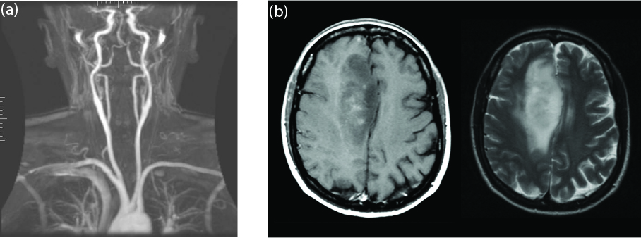
Fig. 3.3 Examples of images obtained with MRI. (a) MRI angiography, view of the arteries in the upper body [11]. (b) MRI of the brain, visualized with different techniques: T1-weighted contrast, where the magnetization is in the same direction as the applied magnetic field (left) and T2-weighted contrast, where the magnetization is perpendicular to the applied magnetic field (right). There is a large tumor in the brain, which is darker in the left image, and much brighter in the right, clearly showing the different tissue composition [12].#
3.5. Addition of angular momenta#
3.5.1. Combining two spin-½ particles#
Angular momenta are vector quantities; when adding and subtracting them, we need to account for this vector nature. To illustrate the complications and the benefits we get from these vector additions, we consider the simplest possible example: the total spin of a composite particle that consists of two spin-½ particles (e.g. a hydrogen atom in the ground state, with angular momentum zero (\(l=0\)), consisting of a proton and an electron, both spin-½ particles). Each of the particles has two possible states, which we’ll call ‘spin up’ and ‘spin down’ as before. For the combined state, we then expect to find four options:
Although these two particles are in a composite state, they are still quantum particles, and therefore the composite state should be a quantum state itself, characterized by quantum numbers. However, we quickly run into trouble if we try to calculate the \(m_s\) quantum number of the combined states given above. For the ‘double up’ and ‘double down’ states we find \(m_s = \frac12 + \frac12 = 1\) and \(m_s = -\frac12 - \frac12 = -1\), respectively, but the middle two options both give \(m_s = 0\). As two different quantum states cannot have the same quantum numbers, we have arrived at a paradox. To resolve it, we need to realize that the spin operators acting on these composite states are themselves composites as well. We found the value of the \(m_s\) quantum number through addition, which is correct, because the composite \(\hat{S}_z\) operator is simply the sum of the two spin-½ \(\hat{S}_z\) operators, or
where \(\hat{S}_z^{(1)}\) acts only on the first particle (say the electron) and is indifferent to the second, while the opposite holds for \(\hat{S}_z^{(2)}\). Now, to go from a ‘spin up’ to a ‘spin down’ eigenstate, we used the lowering operator \(\hat{S}_-\). This operator too becomes a composite, similar to \(\hat{S}_z\) in equation (3.68). Applying it to the ‘double up’ combined state, we do not find either of the middle states, but a linear combination of them:
Equations (3.69) tell us that there is a triplet of composite spin states, which are transferred one into the other by the lowering (and, in the opposite direction, the raising) operators \(\hat{S}_\pm\). Properly normalized, this triplet of states consists of
The three states of the triplet have \(s=1\), and values of \(m_s\) running between \(s\) and \(-s\), as we would expect for angular momentum states. The triplet kind of solves our paradox, but we are still one state short, as the two ‘middle’ options in (3.67) are mutually orthogonal, so we need there to be four states in total. The fourth state is the linear combination of these states that is orthogonal to the \(\Ket{1 0}\) combination in the triplet; it is known as the singlet spin state
The singlet state obviously has \(m_s = 0\) (simply apply the composite \(\hat{S}_z\) operator to it), but also \(s=0\), which we can see in one of two ways: either by applying the composite \(\hat{S}^2\) operator (which gives \(0\)), or by trying to ‘raise’ or ‘lower’ the state with \(\hat{S}_\pm\) (which also give \(0\), i.e., there is only one state on the ‘ladder’). Unlike for the single particle or for the orbital angular momentum, the combined states thus have multiple ladders; in this example there are two, one in which the spins are in parallel (giving a composite particle with \(s=1\)) and one where they are antiparallel (resulting in a composite particle with \(s=0\)).
Composite particles are everywhere. Not only atoms are composites of multiple spin-½ particles, so are atomic nuclei (except, obviously, the single-proton hydrogen nucleus), and nuclear particles themselves (protons and neutrons both consist of three spin-½ particles known as quarks, see Chapter 6). Particles need not be composed of spin-½ particles; they could also be composed of particles with different spin. We can however extend the treatment of the two spin-½ particles easily to either multiple particles or particles with different spins. By induction, we find that combining particles with spins \(s_1\) and \(s_2\) yields multiple possibilities for the composed particles, with spin quantum numbers \(s\) ranging between \(|s_1 - s_2|\) and \(s_1 + s_2\) in integer steps, and as always, associated \(m_s\) quantum numbers ranging from \(-s\) to \(+s\) in integer steps.
As spin and orbital angular momenta are ultimately the same physical quantities, we can also define a total angular momentum, usually denoted by \(\hat{\bm{J}}\), as the (vector) sum of the orbital and spin angular momentum:
The addition rules that give the quantum numbers for the total angular momentum (\(j\) and \(m_j\)) are the same as those for adding spin quantum numbers.
Once we go beyond adding spin-½ particles, a general combined state \(\Ket{s m_s}\) will be a linear combination of composite states \(\Ket{s_1 s_2 m_1 m_2}\):
Working out the prefactors in the combinations (known as the Clebsch-Gordan coefficients) can be a quite time-consuming and tedious (though straightforward) task. To help us out, they have been tabulated for us by physicists of Christmas past (see e.g. Bohm [Boh86], Griffiths and Schroeter [GS18], or Hagiwara et al. [HHN+02]; naturally, they can also be found on Wikipedia [Wik23]).
3.5.2. Mathematical interlude: product state space#
In the example of Section 3.5, it probably didn’t surprise you that we found four options for the possible combinations of two spin-½ particles. After all, each of the particles has two possible states, and \(2 \times 2 = 4\). The combinations we got (the singlet and triplet states) might not be what you had expected, but at least there are four of them, and they are mutually orthogonal. To check that last statement, remember that the first of the two spins in each of the kets is the state of particle 1 and the second that of particle 2, so if we for instance calculate the inner product between the ‘double up’ and the central triplet state, we get
where as before the superscripts indicate which particle we’re talking about. The orthogonality between all other pairs follows in the same way.
For wave functions, we introduced the Hilbert space of all allowed quantum states in Section 1.4.1, and we found that the eigenstates of the Hamiltonian form a basis for this Hilbert space; we get a similar space of functions for any Hermitian operator, with its eigenfunctions as a basis. For operators with a finite, discrete spectrum, these state spaces can be written as vector spaces, with the operators cast in matrix form, and the eigenstates becoming eigenvectors, as we have done for the spin-½ particles in Section 3.4. The combined space of eigenstates of two such operators then becomes the product state space. Product state spaces are not limited to operators with finite, discrete spectra; you can also create product state spaces of Hilbert spaces (as we’ll do when looking at multiple electrons later on) or between a finite-dimensional and an infinite-dimensional state space, for example when considering both the spin and the position state of an electron in a hydrogen atom.
To characterize the product state space, it suffices to define its basis; as the product space will again be a vector space, all its elements can then be written as linear combinations of the basis. To make things concrete, let’s say we have state spaces \(S_A\) and \(S_B\) (to juice things up a bit, rather than calling the systems ‘system A’ and ‘system B’, people often refer to them as Alice’s and Bob’s system, especially when using these states for quantum communication). The product space is then formally written as \(S_{AB} = S_A \otimes S_B\), where the symbol \(\otimes\) is known as the tensor product. The tensor product differs from the Cartesian product \(S_A \times S_B\), which is simply the collection of all pairs \((a,b)\) with \(a \in S_A\) and \(b \in S_B\). For the tensor product, we also define the basis, which we construct from the basis vectors of \(S_A\) and \(S_B\), again using a tensor product. Writing the basis vectors (or states) of \(S_A\) and \(S_B\) as \(\Ket{a}\) and \(\Ket{b}\), the basis of \(S_{AB}\) then consists of elements of the form
To understand what the tensor product in (3.75) means, we go back to a regular vector space, \(V\). An element of \(V\) can be written as a vector, \(\bm{v}\), which, in Dirac notation, becomes a state, \(\Ket{\bm{v}}\). Each vector defines a linear map from the vector space to the (real or complex) numbers, through the inner product. In mathematical notation, given a vector \(\Ket{\bm{v}}\), we have a function \(\phi_{\bm{v}} : V \to \mathbb{C}\) defined as
By the properties of inner products, \(\phi_{\bm{v}}\) is linear (see Section 7.1). The tensor product in (3.75) now defines a bilinear map, taking two arguments, one from \(S_A\) and one from \(S_B\). The bilinear map is defined as the product of the inner products, as you would expect. In particular, if we have an element \(\Ket{ab}\) of \(S_{AB}\), and elements \(\Ket{c} \in S_A\) and \(\Ket{d} \in S_B\), we have
While the above definition is very formal, you have already applied it (tacitly) in equation (3.74); essentially, the elements of the product space act on the elements of the component states.
3.5.3. Product states and entanglement#
A general spin state can be written as a linear combination of a spin-up and a spin-down state (cf. equation (3.43)). If we have two spin-½ particles (one for Alice and one for Bob), they can both be in such linear combinations:
where \(\chi_A\) and \(\chi_B\) should be properly normalized. The product state describing the combined system in \(S_{AB}\) can now be written as
As you can check easily, if \(\chi_A\) and \(\chi_B\) are normalized, the product state in equation (3.79) is normalized as well.
A key property of product states is that the two constituent parts remain independent of each other. If Alice decides to measure the \(z\)-component of the spin of her particle, she will force it to choose between up and down, and change the state of her particle accordingly, but Bob’s particle will remain unaffected.
At this point, I wouldn’t blame you for being a bit confused: in Section 3.5 I argued that while the product states \(\Ket{\uparrow \uparrow}\) and \(\Ket{\downarrow \downarrow}\) are perfectly acceptable, the states \(\Ket{\uparrow \downarrow}\) and \(\Ket{\downarrow \uparrow}\) are not properly characterized by unique quantum numbers. However, in equation (3.79) they seem to have made a comeback, as part of the basis of \(S_{AB}\). Of course, the combination of the three triplet and one singlet state also form a basis, just a different one, and while from a physics perspective we have a clear preference for that one, mathematically it doesn’t matter which basis we work in. To see why, note that product spaces are more than the sum (or rather, the product) of their parts. Any linear combination of the four basis elements is an element of the product space, and so we can write a general element of \(S_{AB}\) as
The state \(\Ket{\bm{\gamma}}\) is thus characterized by four complex numbers \(\gamma_{ij}\). Naturally, if it is to represent a quantum mechanical state, it should still be normalized, so we have:
It is easy to see that there must be more states in \(S_{AB}\) than just product states. While the product states are characterized by four (in general complex) numbers of the form \(\alpha_i \beta_j\), these numbers have two constraints, because both \(\chi_A\) and \(\chi_B\) need to be normalized. The four complex numbers \(\gamma_{ij}\) only have one constraint though, given by the normalization of the state \(\Ket{\bm{\gamma}}\). Therefore, there is ‘room’ for states that are not product states, and these indeed exist[13].
A composite state that cannot be written as a product state is called a mixed state. Such mixed states are entangled: the underlying composite states cannot be separated anymore. Entanglement comes in degrees; we’ll see how we can determine the amount of entanglement. The singlet \(\Ket{00}\) and ‘intermediate triplet’ state \(\Ket{10}\) are examples of maximally entangled states. Entanglement has an immediate consequence in physics. If Alice and Bob each hold a spin-½ particle that together are in an entangled state, a measurement by Alice on her particle will not only affect that particle, but also Bob’s! To see how this works, suppose the particles are in the singlet state, and Alice measures the \(z\)-component of the spin of her particle. She can get ‘up’ (really \(+\hbar/2\)) and ‘down’ (really \(-\hbar/2\)) with equal probability, but after the measurement, her particle will for certain be in that state. However, if Alice’s spin is in the ‘up’ state, we know that Bob’s has to be in the ‘down’ state, and vice versa. Moreover, it doesn’t matter if the two spins are sitting side-by-side, or if Alice first took hers on a trip to the far side of the world; once she measures the spin of her particle, Bob’s immediately assumes the opposite value. This ‘spooky action at a distance’ has spooked many physicists and philosophers, not in the least Albert Einstein, who would have none of it, instead claiming that there should be a ‘hidden variable’ by which the value of the spin of Alice’s and Bob’s particles should be set from the moment they got entangled. As we’ll discuss later, Einstein’s own thought experiment to prove the existence of such a hidden variable was later extended to prove that it in fact cannot exist, and the latter result has been experimentally verified. Quantum particles really get entangled, and the entanglement holds no matter how far apart the particles are.
3.5.4. The density matrix#
If we measure the energy, the magnitude and \(z\)-component of the orbital angular momentum, and the \(z\)-component of the spin of the electron in a hydrogen atom, we know all there is to know about that electron. We’ve found all the relevant quantum numbers describing its state, and we know that after all these measurements, it’s in an eigenstate of all corresponding operators. Such a maximally-determined state is known as a pure state in quantum mechanics. In contrast, a state in which one or more of the quantum numbers are undetermined is known as a mixed state.
3.5.4.1. Pure states#
Both pure and mixed states can be represented by a density matrix, though as you can also represent pure states in other forms (namely as eigenfunctions of the corresponding operators), the formalism of the density matrix is mostly useful for mixed states. However, to define it, we’ll start from a pure state. Suppose we have a pure state \(\Psi\), written in Dirac notation as \(\ket{\Psi}\). We can then define the density operator \(\hat{\rho}\) as the projection on \(\Psi\) (c.f. the definition of the projection operator in equation (1.61)):
Note that the density operator is simply the projection on \(\ket{\Psi}\). If the Hilbert space of our quantum system has a basis \(\{\ket{e_j}\}\), we can define the matrix elements of the density operator (see equation (1.57)) as
The density operator (denoted \(\hat{\rho}\)) and the corresponding density matrix (simply denoted \(\rho\)) of a pure state have three useful properties: they’re Hermitian (\(\rho^\dagger = \rho\)), idempotent (like the projection operator), i.e. \(\rho^2 = \rho\), and have unit trace:
From the density matrix, we can moreover calculate the expectation value of any observable \(\hat{A}\). To do so, we use the fact that the identity operator can be written as the sum over the projections on all basis vectors (equation (1.60))), and write:
Finally, the time evolution of the density operator (i.e., the Schrödinger equation in terms of \(\hat{\rho}\), see Exercise 3.6) is given by
3.5.4.2. Mixed states#
A mixed state cannot be written as a single function in the Hilbert space of our quantum system. Note that this property makes a mixed state different from a superposition state. A superposition state is written as a linear combination of other states, but itself is still a single function in the Hilbert space. A mixed state is not a single state, but a mixture of possible states. To represent it, we’ll use the density operator and density matrix.
In a mixed state, there are multiple states \(\ket{\Psi_k}\) that the system can be found in after a measurement, each with an associated probability \(p_k\). If our system is in a mixed state, we can still calculate the expectation value of any observable via its associated operator, using the standard way of calculating the expectation value, by weighing each option by the associated probability. Therefore, for an operator \(\hat{A}\), the expected outcome of a measurement if the system is in a mixed state is given by:
Comparing equation (3.87) with its pure state equivalent (3.85), we see that we can again write \(\hat{A} = \mathrm{Tr}(\rho A)\) if we generalize the definition of the density operator (3.82) to
For the elements of the corresponding density matrix we then find
The density matrix of a mixed state, like that of a pure state, is Hermitian and has unit trace (equation (3.84)). It can be used to calculate the expectation value of an operator directly through the trace, like in equation (3.85), so \(\Braket{\hat{A}} = \mathrm{Tr}(\rho A)\). Its time evolution is moreover still given by equation (3.86). However, the density matrix of a mixed state is not idempotent: \(\hat{\rho}^2 \neq \hat{\rho}\), which (especially in the matrix representation), gives us a quick way of determining whether a state is mixed or pure.
3.5.4.3. Example: Singlet state#
The singlet combination state of two spin-½ particles is a pure state in the Hilbert space of the joint particles. To be precise, it can be written as a linear combination of two of the states that together form a basis, namely \(\ket{\uparrow \downarrow}\) and \(\ket{\downarrow \uparrow}\). However, each of the individual particles is not in a pure state, as we do not know whether it’s spin is up or down. We can describe both the pure state and the mixed state with a density matrix.
For the pure state, the full basis is \(\left\lbrace \ket{\uparrow \uparrow}, \ket{\uparrow \downarrow}, \ket{\downarrow \uparrow}, \ket{\downarrow \downarrow}\right\rbrace\), and the state[14] can be written in this basis as \(\ket{\chi} = \frac{1}{\sqrt{2}} \left(\ket{\uparrow \downarrow} - \ket{\downarrow \uparrow}\right)\). We could calculate the components of the corresponding density matrix with equation (3.83), but it’s more efficient to use the (3.82), which gives
It’s an easy exercise to check that this density matrix is Hermitian, has unit trace, and is idempotent (\(\hat{\rho}^2 = \hat{\rho}\)), as it should be for a pure state.
For either of the spin \(\frac12\) particles, the probability of being in the spin up and spin down states are \(\frac12\). Therefore, taking (as usual) \(\ket{\uparrow}\) and \(\ket{\downarrow}\) as our basis, we get for their individual density matrices
These matrices are again Hermitian and have unit trace, but are not idempotent, as \(\hat{\rho}^2 = \frac12 \hat{\rho}\).
3.5.5. The EPR paradox and Bell’s inequality#
From a philosophical point of view, people have objected to the concept of entanglement. The most famous opponent no doubt was Albert Einstein himself, who (supposedly) said that ‘God does not throw dice’: Einstein believed that the universe is ultimately deterministic, in the sense that, although the wavefunction of a particle can only tell us something about the probability of the outcome of a certain measurement, the outcome is already determined by the particle’s initial conditions. According to Einstein, the fact that the wavefunction does not contain this information, does not mean that quantum mechanics is wrong (Einstein did not dispute the outcome of either the quantum mechanical calculations nor the associated experiments), but that it is incomplete: there should be a larger theory, of which quantum mechanics would somehow be a subset, which would allow us to calculate all properties of a particle from its initial conditions. As quantum mechanics clearly does not contain all necessary information about the particle to do so, there should be additional variables that contain the missing information. These variables have become known as hidden variables, and the philosophical point of view that the properties of a particle are determined by their initial condition the realist position. In contrast, the (now generally accepted) view that the outcome of the measurement of a physical property of a particle is determined only at the moment of measurement, corresponding to a collapse of the wavefunction, is known as the Copenhagen interpretation, after the city in which Niels Bohr lived and worked.
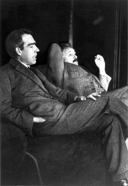
Fig. 3.4 Niels Bohr (left) and Albert Einstein photographed by fellow theoretical physicist Paul Ehrenfest in Ehrenfest’s home in Leiden on 11 December 1925 [15]. Bohr and Einstein both were friends of Ehrenfest and frequently stayed at the house of Ehrenfest and his wife Tatyana Afanasyeva, discussing physics and playing music together. The house, desgined by Afanasyeva, still stands. Ehrenfest and Afanasyeva organized colloquia for graduate students in their home, where guests like Bohr and Einstein gave talks about the latest developments in physics. Afterwards, the lecturers were invited to sign the wall (initially only if Ehrenfest thought the lecture was good). These colloquia later moved to a lecture hall in Leiden university, and continue to be organized today, having collected over the years a very impressive list of signatures on the wall that has been moved with the physics department from one location in Leiden to the next.#
Together with fellow physicists Podolsky and Rosen, Einstein published a paper in 1935 about a thought experiment that has become known as the EPR paradox [EPR35]. The experiment was designed to support their realist position. The argument is simple. Suppose a pair of particles is created in an entangled state, let’s say the singlet spin state. Then, according to the Copenhagen interpretation, the spin of each of the particles is undetermined until one of them is measured. Because the joint state is known, a measurement on one particle will also fix the outcome of a measurement on the other particle: if the first measurement yielded spin up, the second must give spin down. On this point, the correlation between the two measurements, everybody agrees, as it is a prediction based on the theory of quantum mechanics, independent of the interpretation. However, Einstein, Podolsky and Rosen argued, if the Copenhagen interpretation is correct, information must travel from one particle to the other at the time of measurement. From (special) relativity we know that no information can travel faster than the speed of light. But there’s nothing preventing us from first taking the particles very far apart, and then doing the measurements only after the separation, so close together in time that information, even at the speed of light, could not possibly travel from one location to the other. The measurements on each particle would give a seemingly random outcome, but when compared, they would always anti-correlate. Therefore, the Copenhagen interpretation violates the principle of locality (which states that no information can travel faster than light). Instead, the outcome of the measurement should have been determined at the point when the particles were created (or when they became entangled), and therefore one particle already had spin up, and the other spin down, from the outset. The measurement only serves to determine the value, but (again, according to Einstein, Podolsky and Rosen) does not influence the outcome. That quantum mechanics cannot tell us what the outcome will be is therefore a shortcoming of quantum mechanics, and an indication that a hidden variable does exist.
The argument behind the EPR paradox may seem compelling, but ironically, could ultimately be used to do the exact opposite, namely rule out that a hidden variable can exist (or, to be precise, prove that the notion of a hidden variable is incompatible with quantum mechanics). This proof is due to Bell, and now known as Bell’s theorem [Bel64].

Fig. 3.5 Setup of the EPR thought experiment and Bell’s extension of it. (a) Original EPR experiment. A neutral pion with spin 0 decays into an electron-positron pair. Conservation of angular momentum requires that the pair is in a singlet spin combination. The electron and positron travel to locations separated by a large distance. Their spins are then measured, and the results compared. Every time the measurement of the electron spin results in a ‘spin up’, the positron will have ‘spin down’, and vice versa, even though the separation between the measurement locations is so large that information would have to have been transferred faster than the speed of light to communicate the outcome of the measurement. (b) Bell’s modification of the EPR experiment: instead of measuring both the electron and positron spin along the \(z\)-axis, the electron’s spin is measured along direction \(\bm{\hat{a}}\), and the positron’s spin along direction \(\bm{\hat{b}}\); the resulting values are then multiplied and divided by \(\hbar^2/4\), resulting in a sequence of \(+1\) and \(-1\) outcomes.#
To make things concrete, we’ll use a simple thought experiment in the spirit of the EPR paradox that is due to Bohm. A neutral pi meson (also known as a pion, a particle consisting of two quarks (see Chapter 6), for the neutral pi meson either up and anti-up or down and anti-down, making it highly unstable) can spontaneously decay into an electron-positron pair. As the pi meson has spin zero, and angular momentum is conserved, the combined electron-positron system also must have spin zero, and they must therefore be created in the singlet configuration. Working in a reference frame in which the pi meson was stationary, if the electron moves to the right, the positron moves with equal speed to the left. We identify two locations, A and B, where we measure the spin of the positron and electron, respectively. However, unlike in the original EPR thought experiment, we do not measure the spin in the same direction, we measure the component along some (independently set) directions \(\bm{\hat{a}}\) and \(\bm{\hat{b}}\). The outcome of each measurement would still be \(\pm \hbar/2\) (as those are the only possible ones), but the probability of getting each outcome would depend on the direction of \(\bm{\hat{a}}\) and \(\bm{\hat{b}}\). Moreover, if we calculate the product of the two outcomes, we could get either \(- \hbar^2/4\) or \(+ \hbar^2/4\), or, if we measure the outcome in units of \(\hbar/2\), the outcomes can be \(\pm 1\), and so can the products. In particular, if we set \(\bm{\hat{a}} \parallel \bm{\hat{b}}\), we’ll retrieve the original experiment, and always get \(-1\) from the product. Likewise, if we point \(\bm{\hat{a}}\) and \(\bm{\hat{b}}\) in opposite directions (so \(\bm{\hat{a}} \parallel -\bm{\hat{b}}\)), we always get \(+1\). In general, we can define a function \(P(\bm{\hat{a}}, \bm{\hat{b}})\) as the average of the product of the outcomes over many measurements. The special cases above are then \(P(\bm{\hat{a}}, \bm{\hat{a}}) = -1\) and \(P(\bm{\hat{a}}, -\bm{\hat{a}}) = 1\), and in general \(-1 \leq P(\bm{\hat{a}}, \bm{\hat{b}}) \leq 1\).
With a bit more work, we can show that \(P(\bm{\hat{a}}, \bm{\hat{b}}) = - \bm{\hat{a}} \cdot \bm{\hat{b}}\). We define \(S_{\bm{\hat{a}}}^{(1)}\) to be the component of the spin of the positron along the direction of \(\bm{\hat{a}}\), and likewise \(S_{\bm{\hat{b}}}^{(2)}\) as the component of the electron along the direction of \(\bm{\hat{b}}\). We now choose our coordinates such that \(\bm{\hat{a}}\) lies along the positive \(z\) axis (so \(\bm{\hat{a}} = \bm{\hat{z}}\) and that \(\bm{\hat{b}}\) lies in the \(xz\) plane, so \(\bm{\hat{b}} = \sin(\theta)\bm{\hat{x}} + \cos(\theta) \bm{\hat{z}}\), where \(\theta\) is the angle between \(\bm{\hat{a}}\) and \(\bm{\hat{b}}\) (and therefore \(\cos(\theta) = \bm{\hat{a}} \cdot \bm{\hat{b}}\)). In these coordinates, we can calculate the expectation value of product of the measurements of the \(z\) components of the two spins as
which proves the claim that \(P(\bm{\hat{a}}, \bm{\hat{b}}) = - \bm{\hat{a}} \cdot \bm{\hat{b}}\).
Suppose now that Einstein, Podolsky and Rosen were correct, and the complete set of states of the electron and positron indeed depend on a hidden variable \(\lambda\). Also, assume locality, i.e., that, due to their large separation, the outcome of the electron measurement is independent of the positron measurement and vice-versa. Then there exist functions \(A(\bm{\hat{a}}, \lambda)\) and \(B(\bm{\hat{b}}, \lambda)\) that give the outcomes of these measurements. The only possible values these functions can take are \(\pm 1\), i.e., \(A(\bm{\hat{a}}, \lambda) = \pm 1\) and \(B(\bm{\hat{b}}, \lambda) = \pm 1\). Moreover, we have:
and (averaging over many measurements)
where \(\rho(\lambda)\) is the probability density of the hidden variable \(\lambda\). Substituting equation (3.93) into (3.94), we can eliminate the function \(B(\bm{\hat{b}}, \lambda)\):
At this point, Bell introduces a comparison to a third unit vector \(\bm{\hat{c}}\), which will give us the required inequality. He gives no hint as to how he came up with this idea; it may just have been trial and error. But since it works, we will follow along: compare \(P(\bm{\hat{a}}, \bm{\hat{b}})\) to \(P(\bm{\hat{a}}, \bm{\hat{c}})\) where \(\bm{\hat{c}}\) is any other unit vector, which gives:
where in the last equality we used that \(|A(\bm{\hat{b}}, \lambda)|^2 = 1\). Now the product \(A(\bm{\hat{a}}, \lambda) A(\bm{\hat{b}}, \lambda)\) is a number between \(-1\) and \(+1\). Therefore, \(1 - A(\bm{\hat{a}}, \lambda) A(\bm{\hat{c}}, \lambda) \geq 0\), and (by virtue of it being a probability density), \(\rho(\lambda) \geq 0\) as well. Taking the absolute value, we can therefore write
or, using that \(\int \rho(\lambda) \mathrm{d}{\lambda} = 1\),
which is the Bell inequality. As we have not made any assumptions on the hidden variable \(\lambda\), its probability distribution \(\rho(\lambda)\) or the functions \(A(\bm{\hat{a}}, \lambda)\) and \(B(\bm{\hat{b}}, \lambda)\), the inequality should be satisfied for any quantum mechanical theory that includes a hidden variable. Quantum mechanics itself tells us what the function \(P(\bm{\hat{a}}, \bm{\hat{b}})\) is, as we derived in equation (3.92). This result, \(P(\bm{\hat{a}}, \bm{\hat{b}}) = - \bm{\hat{a}} \cdot \bm{\hat{b}}\) is however incompatible with the Bell inequality (3.98), as we can easily show by a counter-example: take \(\bm{\hat{a}} = (1, 0)\), \(\bm{\hat{b}} = (0, 1)\) and \(\bm{\hat{c}} = \frac{1}{\sqrt{2}} (1, 1)\), and we get \(P(\bm{\hat{a}}, \bm{\hat{b}}) = 0\), \(P(\bm{\hat{a}}, \bm{\hat{c}}) = P(\bm{\hat{b}}, \bm{\hat{c}}) = - \frac12 \sqrt{2}\), and thus
We have come to a contradiction. Either quantum mechanics is wrong, and therefore equation (3.92) is invalid, or quantum mechanics is correct, in which case the Bell inequalities are violated, and thus the underlying assumption, the existence of a hidden variable, is wrong. Because quantum mechanics correctly predicts the outcome of a wide range of experimental observations, it is generally held to be correct (Einstein, Podolsky and Rosen agreed with that point), and therefore the hidden variables are ruled out. At the microscopic level, the world is thus indeed stochastic, and moreover nonlocal: the communication between the electron and positron is indeed instantaneous[16]. Luckily, this nonlocality does not violate causality (the concept that a cause always precedes an effect): you cannot use the Bell version of the experiment to submit a message faster than the speed of light. To see why, consider Alice, who gets the electrons, and Bob, who gets the positrons. Alice can measure the spin of the electrons along the direction \(\bm{\hat{a}}\), influencing the measurements Bob will take along direction \(\bm{\hat{b}}\), but Alice has no way of controlling the outcome of her measurements: no matter which direction she picks for \(\bm{\hat{a}}\), the outcome will always be \(\pm \hbar/2\), with a \(50\%\) chance for either result. Therefore, even though Bob can have instantaneous knowledge of the outcome of Alice’s measurements (through aligning his measurement direction \(\bm{\hat{b}}\) with Alice’s \(\bm{\hat{a}}\)), no message was transmitted, since Alice’s results are random.
3.6. General two-particle systems#
As we’ve seen in Section 3.5, if you combine the spins of two spin-½ particles[17] you will get combinations that are either symmetric or antisymmetric, meaning that if you swap the two particles, you will either get the same state, or minus the state. A similar effect applies to the positional part of the state of the particles. For a single particle, the behavior (over time) is described by a wave function \(\Psi(\bm{r}, t)\), which evolves according to the Schrödinger equation (2.58). According to our statistical interpretation (Axiom 1.1), the probability of finding the particle in some volume \(\mathrm{d}^3\bm{r}\) around a point \(\bm{r}\) is given by \(|\Psi(\bm{r}, t)|^2 \, \mathrm{d}^3\bm{r}\). We can easily generalize this notion to a system of two particles: the wavefunction then has two spatial coordinates, defining the positions of the two particles, so we get \(\Psi(\bm{r}_1, \bm{r}_2, t)\), which we interpret to mean that the probability of finding particle 1 in a volume \(\mathrm{d}^3\bm{r}_1\) around \(\bm{r}_1\) and particle 2 in a volume \(\mathrm{d}^3\bm{r}_2\) around \(\bm{r}_2\) is given by \(|\Psi(\bm{r}_1, \bm{r}_2, t)|^2 \, \mathrm{d}^3\bm{r}_1 \, \mathrm{d}^3 \bm{r}_2\). The Hamiltonian of the system with two particles will have two kinetic energy terms (one for each particle), and a potential energy which will depend on the positions of the two particles (and, in general, could depend on time):
where the subscript on each Laplace operator \(\nabla^2\) indicates which of the two particles it acts on (leaving the other one alone). As long as the potential is time-independent, we can separate the temporal and spatial variables, yielding the same time dependence of \(\Psi\) as before, allowing us to write
and leaving us with the time-independent Schrödinger equation to solve.
Some two-particle solutions are direct generalizations of single-particle ones. If we have two different particles (labeled \(1\) and \(2\)) in different states (labeled \(a\) and \(b\)), the combined wave function is simply a product of the single-particle ones:
We’ve already seen an example of what can happen if different particles can potentially be in the same state: they can get entangled. For example, the proton and the electron in a hydrogen atom both have spin-½, and their spin states could get entangled in a spin singlet with total spin zero. However, we will always be able to tell which particle is which; in the example, we could measure either the mass or the charge of one of them to be sure.
Things get really interesting when we consider identical particles. Quantum-mechanical particles can be identical in the way classical ones can never be. Even if you could produce two perfectly spherical billiard balls with the same mass, radius, moment of inertia, surface roughness, and so on, you could always paint one white and one red, and thus tell them apart. In quantum mechanics, two electrons are truly identical; there’s no way of telling which is which. Therefore, no quantum observable should be affected if we swap them; in more mathematical terms, we can say that the quantum observables should be invariant under such swapping operations. The wavefunction however is not an observable. As we’ve just re-asserted above, it’s square is though, and so we must have that for any pair of identical particles, the wave function satisfies
We can take a square root of both sides of equation (3.103), which gives
where \(|\alpha|^2 = 1\). Mathematically, \(\alpha\) can be any complex number with norm \(1\). As it turns out, in three dimensions, physics allows for only two options: \(\alpha = \pm 1\). Particles with \(\alpha = 1\) are known as bosons, while particles with \(\alpha = -1\) are called fermions. Bosons and fermions can be distinguished by their spin: bosons always have integer spin, while fermions have half-integer spin (this result is known as the spin-statistics theorem, from which the limitation of \(\alpha\) to \(\pm 1\) also follows; the proof requires relativistic quantum mechanics). In two dimensions, other values for \(\alpha\) are also possible; in general they are of the form \(\alpha = e^{i \theta}\) with \(\theta \in [0, 2\pi]\). Such (quasi-)particles are known as anions. They occur in the quantum Hall effect, in which conductance is quantified for two-dimensional electron systems in a strong magnetic field and at low temperature.
For identical particles, we cannot write the combined wave function as a simple product state like we did in equation (3.102), but we can write it in general as a linear combination of product states, which obeys the symmetrization requirement:
where we take the \(+\) sign for bosons and the \(-\) sign for fermions. The prefactor \(1/\sqrt{2}\) is to ensure that the state \(\psi_\pm(\bm{r}_1, \bm{r}_2)\) is normalized if \(\psi_a\) and \(\psi_b\) both are.
For bosons, there is no reason why we could not take \(a=b\) in equation (3.105). Multiple bosons can be in the same state, and we need not stop at two. A collection of a large number of identical bosons all in the same ground state is a distinct state of matter, known as a Bose-Einstein condensate. The possible existence of this state was predicted by Bose and Einstein in 1924, but it wasn’t until 1995 before it was first realized in the lab, using ultracold helium nuclei, earning the experimenters the 2001 Nobel prize.
For fermions, the situation is quite different. If two identical fermions (for example two electrons) would be in the same state, equation (3.105) tells us that this state would have a wavefunction which is identically zero. Such a state cannot exist (the probability of finding the particles cannot be zero everywhere). Therefore, two identical fermions cannot occupy the same state. This purely quantum-mechanical result is known as the Pauli exclusion principle. As we will see below, without this effect, chemistry (and therefore life) would not exist.
3.6.1. The helium atom#
A direct application of the the theory of multiple particles is the electrons in any atom that is not hydrogen: they all contain multiple electrons, which are fermions, so the wavefunction that describes their (collective) state should be antisymmetric under swapping any pair of them. The easiest case is helium, with two electrons orbiting a nucleus that contains two protons and (usually) two neutrons. As for hydrogen, the nucleus is much heavier than the electrons, so we’ll work in the approximation that it is fixed. We can then write down the Hamiltonian for the helium atom (i.e., for the wavefunction of the two electrons):
where \(\bm{r}_1\) and \(\bm{r}_2\) are the positions of the two electrons (with the nucleus at the origin), and \(r_1\) and \(r_2\) their respective norms. As shown in the second line, we can write the helium Hamiltonian as the sum of two hydrogen Hamiltonians (one for each electron), plus an extra term representing the electron-electron repulsion. The hydrogen Hamiltonians are slightly different from regular hydrogen, because the nucleus has twice the charge, and therefore the ground state energy (in which we get the square of this charge), becomes four times that of hydrogen itself.
No exact solutions are known of the Schrödinger equation with the helium Hamiltonian. We can however make approximations, some of which will be quite good, as we’ll see in Chapter 5. For now, we’ll start with the crudest possible approximation: ignoring the electron-electron repulsion altogether. In that case, the wave function separates, as \(\hat{H}_{\mathrm{H}_1}\) doesn’t affect particle 2, and vice versa. Therefore, the eigenfunctions \(\psi(\bm{r}_1, \bm{r}_2)\) of the helium Hamiltonian without the electron-electron term can be written as the product of hydrogen eigenfunctions \(\psi_{nlm}(\bm{r})\):
where \(E_1\) is the ground state energy of hydrogen, and the factor \(4\) due to the double charge in the helium nucleus. For the ground state energy (\(n_1 = n_2 = 1\)), we get \(-109\;\mathrm{eV}\), which is pretty far from the actual value of \(-79\;\mathrm{eV}\). The difference of course is not surprising: we ignored electron-electron repulsion, so we expect our estimate to be off significantly.
At this point, you should be protesting: we just asserted above that, because electrons are fermions, they cannot exist in the same state, so surely there should be limitations to equation (3.107). If two electrons are in the same state, they have the same quantum numbers. Orbital wavefunctions are defined by the three quantum numbers \(n\), \(l\), and \(m_l\), so as long as one of them is different between the two, we’re good. However, for the ground state, we have \(n=1\), \(l=0\), \(m_l=0\), so we would be in trouble, except that electrons have a fourth quantum number[18], the spin state \(m_s\). Therefore, the two electrons of the hydrogen atom could both be in a hydrogen-like orbital ground state with \(n=1\), \(l=0\) and \(m_l = 0\), as long as their spins are different. As we’ve seen in Section 3.5, we can’t take one spin up and the other down, but instead will have to combine them into a singlet or a triplet state. Now if the orbital part of the wavefunction (the part described by \(n\), \(l\), and \(m_l\)) is symmetric, the spin part has to be antisymmetric, and so only the singlet will do. Therefore, our approximation of the ground state of helium is the wavefunction \(\psi_{100}(\bm{r}_1) \psi_{100}(\bm{r}_2) \sigma_{-}(1,2)\), with the \(\psi\)’s indicating the orbital part of the wavefunction, and the \(\sigma_{-}\) the singlet spin state.
Of course, we need not put both electrons in the \(\psi_{100}\) state. We could put one of them in an excited state (putting both in an excited state would require more energy than ionizing one of the electrons). Because the orbital states are then different, we can use them to make an antisymmetric combination, allowing for a symmetric spin state, which would be the triplet, as we still need to satisfy the rules for adding angular momenta. We could also make a symmetric combination of the ground state and excited state orbital, made antisymmetric by putting the spins in the singlet. Therefore, there are two qualitatively different ways of getting excited states in the helium atom:
The symmetric orbital (and antisymmetric spin) combination \(\psi_+\) is known as parahelium, and the antisymmetric orbital (symmetric spin) combination \(\psi_-\) as orthohelium. As we’ll see in Section 5.2.1, a symmetric combination of orbitals will on average put identical particles closer together, and an antisymmetric combination will drive them apart, we can predict that for parahelium the interaction term in the Hamiltonian will be higher than for orthohelium, which is indeed the experimentally obtained result.
3.7. The periodic table of elements#
In the previous section, we approximated the combined wavefunction of the two electrons in a helium atom using the solutions of the hydrogen Hamiltonian. We call such hydrogen-orbital based approximate solutions hydrogenic orbitals. We need to complement them with spin states to give the full wavefunction, with the proper antisymmetry property for the fermionic electrons.
When moving from helium to lithium, the third element with three electrons, we cannot construct an approximate ground state from hydrogenic orbitals in the same way we did for helium. There are only two possible spin states for our spin-½ electrons, so adding a third electron with orbital \(\psi_{100}\) is not possible. The two electrons in the helium atom therefore together occupy all possible states with \(n=1\). To add a third electron, we’ll need to put one in an \(n=2\) state. As we’ll see in Chapter 4, higher-order terms make the energy of hydrogen orbitals dependent on not just the principal quantum number \(n\) but also the orbital quantum number \(l\); the state \(\psi_{200}\) then has lower energy than \(\psi_{210}\) (or either of the others with \(l=1\), as the energy won’t depend on \(m_l\) unless we apply a magnetic field). Therefore, our best guess for the ground state of lithium is the ground state of helium together with a third electron in a \(\psi_{200}\) orbital. Naturally, the combined wavefunction will still need to be antisymmetric under exchange of any pair of electrons, but as the orbital state of the added electron is different from the other two, doing so is straightforward. Extending to the fourth element, beryllium, is also not hard: we put the fourth electron in a singlet combination with the third, both in \(\psi_{200}\) orbitals.
By putting two electrons in a \(\psi_{100}\) orbital and two in a \(\psi_{200}\) orbital, we’ve exhausted the \(l=0\) options for \(n=1\) and \(n=2\). The next electron will therefore need to be put in an orbital with \(l=1\). There are three such orbitals, as we now have three choices for \(m_l\). Because we now have \(l=1\), the orbitals have nonzero orbital angular momentum, and the rules for adding angular momenta (of the orbitals and the spin) apply. Therefore, the wavefunction of the fifth electron in boron, the fifth and sixth in carbon, and so on till the tenth electron in neon, will be linear combinations of the possible wavefunctions with \(l=1\) and \(s=\frac12\).
Once we have exhausted all hydrogenic orbitals with \(n=2\), we move on to \(n=3\) for natrium, magnesium, and on till argon with orbitals with \(l=0\) and \(l=1\). However, the nineteenth electron of potassium will not go into a \(n=3, l=2\) orbit, but instead into a \(n=4, l=0\) orbit, as that one turns out to have a lower energy. Only once those two slots are filled, the twenty-first electron of scandium uses an \(n=3, l=2\) orbitals. A similar thing happens with the \(n=4, l=3\) orbitals, which have a higher energy than not only the \(n=5, l=0\) but also the \(n=6, l=0\) orbitals.
Arranging the elements by the highest-energy orbitals their electrons occupy in the ground state, the periodic table emerges. The rows (or ‘period’) correspond to the primary quantum number (at least for the \(l=0\) and \(l=1\) orbitals), whereas the ‘groups’ are set by the orbital quantum number, see Fig. 3.6. The block with \(l=2\) is shifted down one row, and the block with \(l=3\) two rows (these are the lanthanides and actinides, which are usually shown below the table to not make it overly wide). Elements with \(n=8\) have already been found (or rather made in the lab); to date, no elements are known for which the ground state configuration contains an orbital with \(l=4\), but there is no fundamental reason why they could not exist.
As you probably know, chemists refer to the rows in the periodic table as ‘shells’, labeling them with either the principal quantum number, or a corresponding capital letter (the ‘X-ray notation’), where the \(n=1\) shell has a K, \(n=2\) an L, \(n=3\) M, and so on. Shells are divided in subshells, corresponding to the orbital quantum number \(l\). Electrons in the outermost (i.e., highest \(n\)) shell are called valence electrons; unsurprisingly, as their energy is highest, they are the ones that have the weakest binding with the nucleus. Some atoms (predominantly non-metals like carbon, nitrogen and oxygen) can make covalent bonds with other non-metals. In such a covalent bond, valence electrons from the two atoms are entangled into a common orbital, in such a way that each atom effectively has just enough electrons to ‘fill its shell’ to capacity. Therefore, even though oxygen has six electrons in \(n=2\) orbitals, it only can form two ‘covalent links’ to other atoms, while carbon, with four valence electrons, can form four covalent bonds. Helium, neon, and the other elements in the rightmost column of the table already have a full highest shell, and are therefore chemically inert; they are the noble gases. Going down to less filled shells, we run out of valence electrons to completely fill up a shell, and atoms instead arrange in a periodic lattice, sharing electrons between many atoms; these materials therefore form electrically conducting metals. We will discuss the quantum mechanics behind both covalent bonds and metals in much more detail in Chapter 5.
Next to naming the shells, chemists have also come up with a way to describe the ground-state configuration of the electrons in any atom. This configuration contains two pieces of information. The first we’ve already seen: which hydrogenic orbitals the electrons occupy. These orbitals are characterized by a combination of the principal and orbital quantum numbers, \(n\) and \(l\). For \(n\), the notation simply gives the number, but the \(l\) orbitals historically have been labeled with letters - and not in a alphabetical order. We have \(s\) for \(l=0\), \(p\) for \(l=1\), \(d\) for \(l=2\) and \(f\) for \(l=3\). The combination \(nl\) is written in parentheses, with a superscript of how many electrons it applies to; therefore, for oxygen, we have \((1s)^2 (2s)^2 (2p)^4\), and sulphur gets \((1s)^2 (2s)^2 (2p)^6 (3s)^2 (3p)^4\). ‘Reading off’ this configuration from the periodic table is straightforward. The other piece of information however is harder to obtain: the total orbital, spin, and combined angular momentum of an atom. Writing \(L\) for the total orbital angular momentum, \(S\) for the total spin, and \(J\) for the total angular momentum (which could be anything between \(L+S\) and \(|L-S|\)), the combination is written in a somewhat cryptic way as
For \(L\), letters again replace numbers, now using capitals (the same letters though), and the superscript number doesn’t give you the total spin directly, but the multiplicity, \(2S+1\). To illustrate, the ground state of oxygen has \(S=1, L=1, J=2\), so the corresponding symbol is \({}^3P_2\), while the \({}^2S_{1/2}\) of hydrogen tells you that its ground state (unsurprisingly) has \(S=1/2, L=0, J=1/2\). Elements in the same group (i.e., column) in the periodic table will have the same angular momentum ground state, with the noble gases on the right having the simplest one (\({}^1S_0\)), while iron in group 8 gets something as complicated as \({}^5D_4\).

Fig. 3.6 The periodic table, with principal and orbital quantum numbers of the valence electrons. The principal quantum number \(n\) corresponds to the row number; the orbital quantum number \(l\) depends on the group. Due to electron-electron repulsion and higher-order effects, the \(n=4, l=0\) orbital has lower energy than the \(n=3, l=2\) one, resulting the \(l=2\) orbitals to be ‘bumped down’ one row. A similar thing happens to the lanthanides and actinides with \(l=3\) orbitals. Elements with valence electrons with \(n=8, l=0\) have been made in the lab (elements 119 and 120), and no doubt others will follow in the future. Classification of the elements based on the classification by the American Chemical Society [ACS22], figure adapted from [19].#
To figure out what the ground state configuration of an atom is, would in principle require detailed calculations of the energies of all possibilities, from which you can then pick the lowest one. Fortunately, some common principles can be extracted, which allow us to skip all the math and write down the ground state configuration directly. These principles are known as Hund’s rules, and at least the first two can be understood qualitatively quite easily:
If the electrons have the choice of more than one orbital with equal energy, they will sit in different orbitals, in a configuration that maximizes their multiplicity (and therefore the total spin).
For a given value of the spin, the state with the largest possible value of the total orbital angular momentum (satisfying the total antisymmetry condition) will have lowest energy.
Given \(S\) and \(L\), if the outermost shell is less than or equal to half filled, the term with lowest possible \(J\) will have lowest energy, whereas if the outermost shell is more than half filled, the term with the highest possible \(J\) will have the lowest energy
Naturally, the valence electrons in any atom can also occupy excited states, and transition between states by the adsorption and emission of photons. Therefore, each atom has its own emission spectrum, similar to the one of hydrogen in Fig. 1.4, which acts as an atomic fingerprint. As we’ll see in Chapter 5, the same holds true for molecules.
In contrast to the preceding sections, here we’ve taken a quite rough approximation for the eigenfunctions of the electrons in various atoms. You might wonder how good this approximation is, and if we can do any better. The unsurprising answer to the first question is ‘quite bad’, but the fortunate answer to the second question is ‘yes’. Unfortunately, we’re already out of our depth with regards to analytical methods[20], but there are many approximation methods that can get us much closer to the actual states. One result of those approximation methods is a correction to the hydrogenic orbitals we’ve used for our atoms, in particular for the ground state. These more accurate orbitals are known as Slater-type orbitals, or STOs, given by
where the \(Y_l^m(\theta, \phi)\) are (still) the spherical harmonics, \(a\) is the Bohr radius, and \(A\) a normalization constant. The principal quantum number \(n\) gets replaced by an effective value \(n_\mathrm{eff}\), which is equal to \(n\) for \(n=1, 2, 3\), but reduced for higher values, with \(n_\mathrm{eff} = 3.7\) for \(n=4\), \(n_\mathrm{eff} = 4.0\) for \(n=5\), and \(n_\mathrm{eff} = 4.2\) for \(n=6\). Likewise, the effective charge of the nucleus is reduced due to screening; they differ not just per atom but also per atomic orbital (with lower orbitals having higher values as there are fewer screening electrons). STOs are sometimes used in quantum chemistry software. They have their shortcomings, but are a first step to a more accurate approximation of the actual atomic wave functions.
Fig. 3.7 The periodic table with division into regions according to how and where one might encounter the elements. Cartoon by Randall Munroe, CC-BY-NC 2.5. Source: xkcd.com/2913/ [21].#
3.8. Problems#
Exercise 3.1 (Eigenvalues of the orbital angular momentum operator)
From the algebraic calculations in Section 3.1, we got both integer and half-integer values for the quantum number \(l\). From the solution of the eigenstates of the hydrogen atom, we know however that for orbital angular momentum, we only get the integer values. Thus, in contrast to spin, where, with the same commutation relations, the half-integer values do occur, there must be an extra piece of physics in the orbital angular momentum operator that excludes the half-integer options. That in itself is perhaps not surprising: while we define the spin operators through the commutation relations, for the orbital angular momentum operators we derived the commutation relations from the ‘quantization’ of the classical definition \(\bm{L} = \bm{r} \times \bm{p}\) of the angular momentum. In this problem, we’ll ‘disentangle’ the cross product, ending up with two mathematical equivalents of harmonic oscillators, from which we can prove that we can only get integer values of \(l\). To start, we define the operators
where \(\alpha = a^2/\hbar\), with \(a\) the Bohr radius.
Verify that \([\hat{q}_{+}, \hat{q}_{-}] = [\hat{p}_{+}, \hat{p}_{-}] = 0\) and \([\hat{q}_{+}, \hat{p}_{-}] = [\hat{q}_{-}, \hat{p}_{+}] = i \hbar\).
The result of (a) shows that the \(\hat{q}\)’s and \(\hat{p}\)’s have the same commutation relations as the position and momentum operators. How would you pair the \(\hat{q}\)’s and \(\hat{p}\)’s such that they correspond to ‘orthogonal directions’?
Show that
\[\hat{L}_z = \frac{1}{2 \alpha} \left( \hat{q}_{+}^2 - \hat{q}_{-}^2\right) - \frac{\alpha}{2} \left( \hat{p}_{+}^2 - \hat{p}_{-}^2\right).\]Now show that we can write \(\hat{L}_z\) as the difference between two Hamiltonians describing one-dimensional harmonic oscillators with frequency \(1\) and mass \(m = 1/\alpha\). Hint: Make use of the sets of \(\hat{q}\) and \(\hat{p}\) operators you grouped in (b).
Combine what you know about the eigenvalues of the harmonic oscillator with the result of (d) to prove that the eigenvalues of \(\hat{L}_z\) must be integer multiples of \(\hbar\).
Exercise 3.2 (Solving the hydrogen Hamiltonian with raising and lowering operators)
Derive equation (3.29) for \(\hat{H}_l\) through explicit calculation of \(\hat{A}_l^\dagger \hat{A}_l\).
Show that the commutator of the ladder operator and its Hermitian conjugate is given by
(3.111)#\[\left[ \hat{A}_l, \hat{A}_l^\dagger \right] = \frac{a_0^2 m_\mathrm{e}}{\hbar^2} \left( \hat{H}_{l+1} - \hat{H}_l \right).\]Find the commutator \(\left[ \hat{A}_l, \hat{H}_l \right]\), and use it to prove that \(\hat{A}_l \hat{H}_l = \hat{H}_{l+1} \hat{A}_l\). Hint: you will only need to combine your results of (a) and (b) here.
Prove that if \(u_l(r)\) satisfies equation (3.31) with eigenvalue \(E_l\), then \(\hat{A}_l u_l\) is an eigenfunction of \(\hat{H}_{l+1}\) with eigenvalue \(E_l\).
Show that the last equality in equation (3.33) holds. You may assume that \(u_{l_\mathrm{max}}\) is properly normalized.
Argue why the values of \(l\) in \(u_{nl}\) are restricted to the familiar range \(l = 0, 1, \ldots, n-1\).
By solving the first-order differential equation (3.32) for \(n=1, l=0\), find an expression for \(u_{10}(r)\). You may leave the normalization constant in the expression.
By solving the first-order differential equation (3.32) for \(l=n-1\) and arbitrary \(n\), explicitly find the expression for \(u_{n,n-1}(r)\). Again, you may leave the normalization constant in the expression.
Exercise 3.3 (Orbital angular momentum and kinetic energy)
The operators representing the square and the \(z\)-component of the angular momentum can be expressed in spherical coordinates as
As we derived in class, these operators commute; their joint eigenfunctions are the spherical harmonics \(Y_l^m(\theta, \phi)\), with eigenvalues \(\hbar^2 l (l+1)\) for \(\hat{L}^2\) and \(\hbar m\) for \(\hat{L}_z\) (note that the \(m\) here is the quantum number \(m_l\), not the mass). The fact that the spherical harmonics are the eigenfunctions is not surprising if you compare the expression for \(\hat{L}^2\) with the Laplacian in spherical coordinates; you’ll find that the angular part of the Laplacian is exactly \(-\hat{L}^2 / (\hbar^2 r^2)\). This observation allows us to split the kinetic energy into a radial and an angular part. As the kinetic energy is proportional to the square of the momentum, we need an expression for the radial momentum. Defining[22] ‘operator vectors’ \(\hat{\bm{r}} = (\hat{x}, \hat{y}, \hat{z})\) and \(\hat{\bm{p}} = (\hat{p}_x, \hat{p}_y, \hat{p}_z)\), we might define the radial component of the momentum by the projection of \(\hat{\bm{p}}\) on the unit vector in the radial direction (\(\hat{\bm{r}}/r\), where as usual \(r = \sqrt{x^2 + y^2 + z^2}\)). Unfortunately, this won’t do, as the resulting operator is not Hermitian.
Show that \(\hat{\bm{r}} \cdot \hat{\bm{p}}\) is not Hermitian.
Show that \(\hat{p}_r = \frac{1}{2r} \left(\hat{\bm{r}} \cdot \hat{\bm{p}} + \hat{\bm{p}} \cdot \hat{\bm{r}} \right)\) is Hermitian.
Substituting the recipes for \(\hat{\bm{r}}\) and \(\hat{\bm{p}}\), we find the recipe for \(\hat{p}_r\):
\[p_r = - \frac{i\hbar}{2} \left[ \frac{1}{r} \bm{r} \cdot \bm{\nabla} + \bm{\nabla} \cdot \left( \frac{\bm{r}}{r} \right) \right].\]Note that here \(\bm{r}\) is just the position vector. We can write \(\bm{\nabla}\) in both Cartesian and spherical coordinates, from which we find that \(\bm{\nabla} \cdot \bm{r} = 3\) and
\[\bm{r} \cdot \bm{\nabla} = x \frac{\partial }{\partial x} + y \frac{\partial }{\partial y} + z \frac{\partial }{\partial z} = r \frac{\partial }{\partial r}.\]Use the above expressions to find an expression for \(\hat{p}_r\) in terms of \(r\) and derivatives to \(r\). NB: remember that an operator always acts on a function!
Show that the commutator of \(\hat{r}\) (recipe: multiply with \(r\)) and \(\hat{p}_r\) is the same as the one-dimensional version, i.e., \(\left[ \hat{r}, \hat{p}_r \right] = i\hbar\).
Show that
(3.112)#\[\hat{p}_r^2 = - \frac{\hbar^2}{r^2} \frac{\partial }{\partial r} \left( r^2 \frac{\partial }{\partial r} \right).\]Recognizing equation (3.112) as the radial part of the Laplacian in spherical coordinates, we can write
(3.113)#\[\nabla^2 = - \frac{1}{\hbar^2} \hat{p}_r^2 - \frac{\hat{L}^2}{\hbar^2 r^2}.\]
Exercise 3.4 (Three-dimensional harmonic oscillator)
The Hamiltonian for the three-dimensional harmonic oscillator is given by:
If we write this Hamiltonian in Cartesian coordinates, we see that it separates into three one-dimensional harmonic oscillator Hamiltonians:
where \(\hat{H}_x = (\hat{p}_x^2/2m) + \frac12 m \omega^2 \hat{x}^2\), and similar for \(y\) and \(z\). As these three Hamiltonians commute with each other, the solutions of the Schrödinger equation with the three-dimensional Hamiltonian (3.114) factorize, i.e. they can be written as
where the three functions of \(x\), \(y\) and \(z\) are the solutions to the one-dimensional Schrödinger equation with harmonic potentials.
Argue that the energies of the three-dimensional Schrödinger equation with a harmonic potential are given by
\[E = \left(n_x + n_y + n_z + \frac32 \right) \hbar \omega.\]With equation (3.113), we can also write the three-dimensional Hamiltonian (3.114) in terms of the radial and angular momentum operators:
\[\hat{H} = \frac{\hat{p}_r^2}{2m} + \frac{\hbar^2}{2m r} \hat{L}^2 + \frac12 m \omega^2 \hat{r}^2.\]The angular part of this Hamiltonian is completely covered by the angular momentum operator \(\hat{L}^2\), so we may also expect the solutions to separate into an angular part (which will be the spherical harmonics) and a radial part, for which we can write an effective radial Hamiltonian:
(3.115)#\[\hat{H}_l = \frac{\hat{p}_r^2}{2m} + \frac{\hbar^2 l (l+1)}{2m r} + \frac12 m \omega^2 \hat{r}^2\]The eigenfunctions of this radial Hamiltonian will be functions of \(r\), and be characterized by quantum numbers \(n\) and \(l\). We shall write them as \(R_{nl}(r)\).
Relate the (radial) quantum number \(n\) to the Cartesian quantum numbers \(n_x\), \(n_y\) and \(n_z\).
Find the degeneracy of \(E_n\). Like for the one-dimensional harmonic oscillator, the three-dimensional one has associated raising and lowering operators, defined as
\[\hat{A}_{l, \pm} = \frac{1}{\sqrt{2m\hbar\omega}} \left( \mp i \hat{p}_r - \frac{(l+1)\hbar}{r} + m \omega r \right).\]Unlike for the one-dimensional harmonic oscillator, \(\hat{A}_{l, \pm}\) don’t just change the energy, they also change the angular momentum. In particular, \(\hat{A}_{l, -}\) lowers the energy by \(\hbar \omega\) but raises the angular momentum quantum number \(l\) by \(1\):
\[\hat{A}_{l, -} R_{n, l} = \alpha_- R_{n-1, l+1},\]where \(\alpha_-\) is a normalization constant. Now the eigenstates have two kinds of kinetic energy: radial and tangential. If the angular momentum goes up, so does the tangential velocity and thus kinetic energy; consequently, the \(\hat{A}_{l, -}\) operator must decrease the radial kinetic energy. Therefore, the new orbital is more circular than the previous one. At some point, there will be no radial kinetic energy left, and the angular momentum is maximal; applying the lowering operator once more should then give a zero (as otherwise the radial kinetic energy becomes negative). This ‘lowest rung’ solution, sometimes referred to as a ‘circular orbit’, therefore satisfies (with \(\mathcal{L}\) representing the maximum value of \(l\)):
(3.116)#\[0 = \hat{A}_{\mathcal{L},-} R_{0, \mathcal{L}} = \left( \frac{\partial }{\partial r} + \frac{1}{r} - \frac{\mathcal{L}+1}{r} + \frac{m \omega}{\hbar} r \right) R_{0, \mathcal{L}}\]Find and sketch the function describing the circular orbit (i.e., the solution of the ordinary differential equation (3.116)).
Exercise 3.5 (An electron in an oscillating magnetic field)
In class, we studied what happened when an electron (with spin \(\frac12\)) is placed in a constant magnetic field. If the electron is at rest, we get a simple Hamiltonian, coupling the (externally applied) field \(\bm{B}\) to the spin vector \(\bm{S}\) of the electron, through the electron’s magnetic dipole moment \(\bm{\mu} = \gamma \bm{S}\):
In particular, if we define the direction of the external field as the \(z\)-direction (so \(\bm{B} = B_0 \bm{\hat{z}}\)), the field will couple to the \(z\) component of the electron’s spin, and the Hamiltoinan becomes
We found that in this setup, the expectation value of the particle’s spin, \(\Braket{\bm{S}}\), will precess around the \(z\) axis with Larmor frequency \(\omega_\mathrm{L} = \gamma B_0\). In this problem, we’ll generalize this system to the case that the magnetic field is oscillating, i.e., we have
NB: the oscillation frequency \(\omega\) is not to be confused with the precession frequency \(\omega_\mathrm{L}\). Suppose we initialize the system such that the electron is in the spin-up state with respect to the \(x\) (not \(z\)!) axis, i.e., the initial spinor is
Solve the (time-dependent!) Schrödinger equation for the evolution of the spinor over time, i.e., solve
\[i \hbar \frac{\partial \chi}{\partial t} = \hat{H}(t) \chi,\]where \(\hat{H}\) is given by equation (3.118) and the initial condition of the spinor is equation (3.120).
Show that the (time-dependent) probability of getting \(-\hbar/2\) if you measure \(\hat{S}_x\) is given by
\[\sin^2\left(\frac{\gamma B_0}{2 \omega} \sin(\omega t) \right).\]Find the minimum field strength \(B_0\) necessary to force a complete flip in \(\hat{S}_x\).
Exercise 3.6 (Properties of the density operator)
In this problem we’ll prove some of the properties of the density operator given in Section 3.5.4.
Show that for a pure state, the density operator is idempotent, i.e., \(\hat{\rho}^2 = \hat{\rho}\).
Through explicit calculation, show that the trace of the density matrix is one for any state, i.e., \(\mathrm{Tr}(\rho) = 1\).
Prove that the time evolution of the density operator is given by equation (3.86) for any state, as long as the probabilities associated with the state are independent of time. Hint: Use the product rule to calculate
\[i \hbar \frac{\mathrm{d}\hat{\rho}}{\mathrm{d}t} = i \hbar \frac{\mathrm{d}}{\mathrm{d}t} \left(\sum_k p_k \Ket{\Psi_k}\Bra{\Psi_k}\right)\]and the Schrödinger equation to evaluate the time derivative of \(\Psi_k\).