
2. Solutions to the Schrödinger equation#
2.1. The time-independent Schrödinger equation#
The full Schrödinger equation (1.12) is a partial differential equation, as it involves derivatives to both time and space. Finding general solutions to partial differential equations is often difficult. However, for the case that the potential \(\hat{V}\) is independent of time, we can use separation of variables to reduce the equation to two ordinary differential equations, in time and space separately; from the solutions of these ordinary differential equations we can then construct the general solution to the partial differential equation.
The first step in separating variables is to look for a solution that can be written as a product of two functions, one of time and one of space. We’ll use a lowercase psi, \(\psi(x)\), for the space-dependent function, and an uppercase phi, \(\Phi(t)\), for the time-dependent one. Substituting \(\Psi(x, t) = \Phi(t) \psi(x)\) into the Schrödinger equation (1.12) we get
We can now divide both sides of equation (2.1) by the product \(\Phi(t) \psi(x)\), which gives
Note that in equation (2.2), the left-hand side only depends on time, while the right-hand side only depends on space. That means that if we change the time but stay at the same place, the right-hand side doesn’t change, so neither can the left-hand side. Likewise, if we compare two positions at the same time, the left-hand side doesn’t change, so neither can the right-hand side. Therefore, both sides must be equal to some constant. For later purposes, we’ll call this constant \(E\). Consequently, we can write equation (2.2) as two separate ordinary differential equations:
We multiplied equations (2.3)a and (2.3)b by \(\Phi(t)\) and \(\psi(x)\) again to make them more readable. Equation (2.3)a is a first-order differential equation that can be solved easily (see Section 7.4.1); the solution is given by
where \(A\) is an integration constant. Because the final solution, \(\Psi(x, t) = \Phi(t) \psi(x)\) must be normalized, and we’ll get an integration constant in \(\psi(x)\) as well, we can set \(A\) to \(1\) here.
The solution of equation (2.3)b will depend on the choice of the potential function \(V(x)\). We will work out some examples in Section 2.2. You may have noticed that the left-hand side of equation (2.3)b is simply the Hamiltonian operator \(\hat{H}\), equation (1.19), applied to the space-dependent part of the wavefunction, \(\psi(x)\), which allows us to write the equation as
Equation (2.5) is known as the time-independent Schrödinger equation. The solutions to this equation are pairs of eigenfunctions[1] \(\psi(x)\) and eigenvalues \(E\) of the Hamiltonian operator \(\hat{H}\). As the Hamiltonian represents the energy of the system, you’ll understand why we chose to label the constant in equation (2.3) as \(E\).
In general, we will find a collection of solutions of equation (2.5). The spectrum (collection of eigenvalues) could be discrete, continuous, or a combination of both. If the spectrum is discrete, we can label the solutions and their eigenvalues by integers; in one dimension, that will be a single integer for which we usually will use the letter \(n\). The solutions are then given as combinations (\(\psi_n(x)\), \(E_n\)). For each of the solutions \(\psi_n(x)\), we have a corresponding time-dependent part \(\Phi_n(t) = \exp(-i E_n t / \hbar)\). By Axiom 1.4, the general solution to the time-independent Schrödinger equation can then be written as a sum over the eigenfunctions[2] of the Hamiltonian:
Given an initial condition, i.e. a wavefunction \(\Psi(x, 0)\) at \(t=0\), we can determine each of the \(c_n\) values using the orthogonality of the eigenfunctions (Lemma 1.2):
We will get examples of discrete spectra for the infinite well and the harmonic potential, as well as for the bound states of hydrogen. If the spectrum of the Hamiltonian is continuous, we can also write the general solution in terms of the eigenfunctions, but now the sum becomes an integral, and the coefficients become functions of space; we will work out the details when considering the free particle. In both cases, the eigenstates of the Hamiltonian have two more properties. First, they are stationary states. Although the full wavefunction \(\Psi(x, t)\) is time-dependent, the probability density \(|\Psi(x, t)|^2\) is not, because the time-dependent part is a complex exponential:
Consequently, all probabilities and all expectation values of particles in an eigenstate are time-independent. Second, the eigenstates have definite energy, which is simply an application of the fact that the energies are the eigenvalues of the Hamiltonian (see Section 1.4.3). We can easily verify this statement, as we have
and
so
2.2. Some one-dimensional examples#
2.2.1. The infinite square well#
As our first example, we’ll consider a potential that is utterly unrealistic, but nicely illustrates some of the quantum effects while keeping the maths (relatively) simple. This example is known as the (one-dimensional) infinite square well potential, defined as
As long as the particle is inside the well (\(0 < x < a\)), it’s potential energy is zero; outside the well it’s potential energy is infinite. Therefore, the particle will be constricted to the well. The Hamiltonian inside the well is simply the kinetic energy; finding the eigenfunctions of that energy is a straightforward exercise. We have
or, defining \(k = \sqrt{2 m E / \hbar^2}\) and rearranging terms
Mathematically, equation (2.14) is identical to the equation for a harmonic oscillator in classical mechanics. Its solutions can be written either as sines and cosines, or as complex exponentials. Taking the first approach, we have for the general solution to (2.14):
where \(A\) and \(B\) are integration constants, to be determined by the boundary conditions. Because the potential is infinite outside the well, we must have \(\psi(x) = 0\) for \(x<0\) or \(x>a\). We demand that \(\psi(x)\) is continuous; if not, we’d also get a discontinuity in our probability density. Therefore
and
While equation (2.16) simply gives \(B=0\), equation (2.17) gives us a collection of possible values for \(k\), which in turn determine the eigenvalues \(E\). Equation (2.17) is satisfied for any value \(k = n \pi / a\), where \(n\) is an integer. For physical reasons, we cannot have \(n=0\), as then the solution would be \(\psi(x) = 0\), which is not normalizible (the particle has to be somewhere). As \(\sin(x) = -\sin(-x)\), we can also exclude the negative values of \(n\), as the probability density goes with the square of \(\psi\) and thus we won’t be able to distinguish between the solution for \(n\) and \(-n\). Therefore, the solutions to the time-independent Schrödinger equation with the infinite well potential are given by
Note that the solutions are pairs of eigenfunctions and corresponding eigenvalues. We still need to determine the value of the integration constants \(A_n\) (which in principle can depend on \(n\), though in this case they won’t); these are set by the normalization condition (1.10):
In principle, \(A_n\) could contain a complex part, which we intrinsically cannot determine as we cannot measure \(\psi(x)\) directly. This complex part is known as the phase of the wavefunction; we can write any complex number \(A\) as a magnitude times a phase factor:
As we cannot determine the phase, we’ll usually take the magnitude of the integration constant for the normalization factor; in this case we find that \(A_n = \sqrt{2/a}\) for all values of \(n\).
In the calculation above, we found the possible energy eigenvalues of the Hamiltonian for a particle in an infinite square well. As we’ve asserted in Axiom 1.3, a measurement of the energy of such a particle will always yield an eigenvalue of the Hamiltonian. Therefore, the possible energies of the particle are quantized: only specific values are allowed, all values in between are explicitly excluded. This quantization is what gives quantum mechanics its name, and is a clear distinction from classical mechanics, where there is no reason the particle inside the well could not have a specific energy. In particular, the quantum particle will always have a nonzero energy, because the lowest eigenvalue is nonzero. As the energy inside the well is kinetic energy only, this implies that a quantum particle in such a well cannot be standing still, in correspondence with the Heisenberg uncertainty principle; after all, a particle that would stand still has a definite position and a definite (namely zero) momentum.
The eigenfunction corresponding to the lowest energy eigenvalue is known as the ground state. The other eigenfunctions are known as excited states. The ground state and excited states closely correspond to the fundamental and higher-order modes of waves in a string; for the current example, they are mathematically identical. The first few eigenstates of the square well are plotted in Fig. 2.1.

Fig. 2.1 The first few eigenstates of the one-dimensional Hamiltonian with an infinite square well potential. The eigenstates are simply the sines which are zero at both sides of the well; while the ground state \(\psi_1(x)\) has no nodes inside the well, the excited states have increasing numbers of nodes, where the probability of finding the particle equals zero. Eigenstates have been shifted vertically to show them more clearly, for each the corresponding dashed line represents \(\psi = 0\).#
It is a straightforward exercise to verify that the eigenstates \(\psi_n(x)\) of the Hamiltonian as given by equation (2.18) are orthogonal (as they have to be by Lemma 1.2). Once the eigenfunctions are normalized, they are also orthonormal, i.e.
In this case, you can also prove that the eigenfunctions form a complete set; the fact that the sines form a complete set is known as Dirichlet’s theorem and is why you can write any function \(f(x)\) as a Fourier sine series. As we’ve seen in Section 2.1, the general solution to the Schrödinger equation will be a linear combination of eigenstates \(\psi_n(x)\) with coefficients \(c_n\). If we then measure the energy of a particle in such an infinite well, by Axiom 1.3 we force it to choose one of the eigenvalues of the Hamiltonian, resulting in a ‘collapse’ of the wavefunction to the corresponding eigenstate. A concrete example may help illustrate these ideas.
Example 2.1 (Particle in an infinite well)
Suppose a particle in an infinite well has an initial wave function given by
and of course \(\Psi(x, 0) = 0\) outside the well. Find (a) the normalization constant \(A\), (b) \(\Psi(x, t)\), (c) the probability that a measurement of the energy of this particle yields the value \(E_2\), and (d) the probability that a measurement of the energy of this particle yields the value \(E_1\).
Solution
We can find the normalization constant \(A\) by imposing the normalization condition (1.10), which gives
\[1 = \int_{-\infty}^\infty \left|\Psi(x,t)\right|^2 \mathrm{d}x = |A|^2 \int_0^a x^2 (a-x)^2 \mathrm{d}x = |A|^2 \frac{a^5}{30},\]so \(A = \sqrt{30/a^5}\).
To find \(\Psi(x, t)\), we need to expand \(\Psi(x, 0)\) in the eigenstates of the Hamiltonian. By equation (2.7), we get the coefficient of the \(n\)th eigenstate by taking the inner product between \(\Psi(x, 0)\) and \(\psi_n(x)\):
\[\begin{split}\begin{align*} c_n &= \Braket{\psi_n(x) | \Psi(x, 0)} = \int_0^a \sqrt{\frac{2}{a}} \sin(\frac{n\pi}{a} x) \sqrt{\frac{30}{a^5}} x (a-x) \mathrm{d}x \\ &= \frac{2\sqrt{15}}{a^2} \int_0^a x \sin(\frac{n\pi}{a} x) \mathrm{d}x - \frac{2\sqrt{15}}{a^3} \int_0^a x^2 \sin(\frac{n\pi}{a} x) \mathrm{d}x \\ &= \frac{4 \sqrt{15}}{n^3 \pi^3} \left[ \cos(0) - \cos(n\pi) \right]\\ &= \begin{cases} 0 & n \;\text{even} \\ 8 \sqrt{15}/(n\pi)^3 & n \;\text{odd} \end{cases} \end{align*}\end{split}\]Given the coefficients, the time-dependent solution is given by equation (2.6), which in this case reads
\[\Psi(x, t) = \sqrt{\frac{30}{a}} \left( \frac{2}{a} \right)^3 \sum_{n\;\text{odd}} \frac{1}{n^3} \sin(\frac{n\pi}{a} x) \exp\left(- \frac{i \pi^2 \hbar^2}{2 m a^2} n^2 t \right).\]As \(c_2 = 0\), the probability of measuring \(E_2\) equals zero.
The probability of measuring \(E_1\) is given by
\[|c_1|^2 = \left|\frac{8 \sqrt{15}}{\pi^3} \right|^2 = \frac{960}{\pi^6} \approx 0.998.\]The probability of measuring \(E_1\) is thus very high, which makes sense if you consider the shape of the function we started with: a parabola with a maximum halfway the well, strongly resembling the ground state.
2.2.2. Free particles#
You might wonder why we bothered restricting the particle to the infinite well in Section 2.2.1. Inside the well, the potential is zero, so wouldn’t it be easier to start with a potential that is zero everywhere? Such a particle is known as a free particle. As we’ll see, there’s a subtlety involved with the absence of boundary conditions that makes the analysis of these particles a bit more tricky; also, the spectrum of energy eigenvalues of these particles will be continuous rather than discrete (and thus not ‘quantized’).
Of course, the differential equation for the free particle is identical to that of the particle inside the well, as in both cases the potential energy is zero. We thus retrieve equation (2.14), but this time we’ll write the solutions as complex exponentials:
Writing the eigenstates in this form, you might recognize that they are the same as the plane wave eigenfunctions of the momentum operator \(\hat{p}\) we found in Section 1.4.3 (see equation (1.39)). This is hardly surprising, as for the free particle, the Hamiltonian is simply the kinetic energy, and the kinetic energy operator is proportional to the momentum squared, \(\hat{K} = \hat{p}^2 / 2m\), so eigenfunctions of the momentum operator become eigenfunctions of the kinetic energy as well. If we have a momentum eigenfunction \(f_p(x)\) with eigenvalue \(p\), we can find its (kinetic) energy eigenvalue by applying the kinetic energy operator to it:
so we unsurprisingly find that \(E = p^2 / 2m\), and \(k = \sqrt{2 m E / \hbar^2} = p/\hbar\). We already encountered this exact same relation in equation (1.2), relating the momentum \(p\) of a particle to its wave number \(k\), as postulated by De Broglie; we now find that this is a direct consequence of the Schrödinger equation. Moreover, we can explicitly write the time-dependent wave function of a free particle as a traveling wave (where those of the particle in a well were stationary, standing waves), as we get
Our plane wave solutions thus consist of a wave traveling to the right (first part) and a wave traveling to the left (second part), both at speed
The shape of the wave doesn’t change. The wave is a function of the combination \(x \pm v t\), so after a time \(t\), the whole wave has shifted a distance \(x = vt\) to the right or left. To simplify the notation, we can allow \(k\) to assume negative values, and write the plane wave for wavevector \(k\) as
Unfortunately, our plane wave solution suffers from the same problem we had with the eigenfunctions of the momentum operator: they are orthogonal but not normalizable, as we get
so the integral becomes infinite. Therefore, just like there are no free particles with a definite momentum (as the eigenfunctions are outside the quantum mechanical Hilbert space), there are no eigenstates with a definite energy. However, the eigenfunctions of the Hamiltonian still form a basis for all functions that are in the Hilbert space, and the general solution to the time-dependent Schrödinger equation can therefore be written as a linear combination of the eigenstates. Because the spectrum is now continuous, this linear combination comes in the form of an integral rather than a sum. The coefficients of the various eigenstates in this integral are usually denoted as functions \(\phi(k)\) rather than \(c(k)\) (which would be more consistent with our earlier notation), which gives the general solution as
Note the similarity with equation (1.42); the only difference is that we now integrate over the wavenumber instead of the momentum. At \(t=0\) equation (2.27) simplifies to the inverse Fourier transform of \(\phi(k)\). Finding the function \(\phi(k)\) from the initial condition \(\Psi(x, 0)\) then boils down to taking the Fourier transform of that function, as we have
The solution given in equation (2.27) is known as a wave packet, a collection of plane waves that together (through mutual interference) gives the particle a finite probability density for a limited range in space. The price is that the particle no longer has a well-defined momentum, but will carry a range of possible momenta, and the more precisely we determine the momentum (meaning a narrower function \(\phi(k)\)), the more spread out the position probability density will be, and vice versa. The plane wave solution itself is the (mathematically valid but unphysical) case where the momentum is precisely defined but the probability of finding the particle anywhere becomes zero.

Fig. 2.2 Wave packets. (a) Interference between two waves with close but not identical wavelengths results in alternating constructive and destructive interference, and the emergence of beats. (b) Wave packets with a carrier wave (blue) ‘supporting’ a modulation (purple). The speed of the carrier wave is known as the phase velocity, \(\omega / k\), while the envelope travels at the group velocity, \(\mathrm{d}\omega / \mathrm{d}k\).#
Wave packets are familiar concepts from classical mechanics. There too, they emerge from wave superposition, for instance by combining two traveling waves with slightly different wavelengths, see Fig. 2.2. The resulting modulation wave can be found as the envelope of the generating waves: it describes how the maximum amplitude of the waves changes. In both classical and quantum mechanics, it is the envelope that carries information, not the generating waves (known in classical mechanics as the carrier waves). Moreover, the envelope and carrier waves travel at different velocities, known as the group and phase velocities respectively. As we’ll see, the velocity we found in equation (2.24) is the phase velocity. To find the velocity, we need the relation between the frequency \(\omega\) and the wave number \(k\) of the wave; this relation is known as the wave’s dispersion relation. Writing the wave in the form \(\exp\left(i (k x - \omega t) \right)\), we can read off from equation (2.25) that the dispersion relation for a plane wave solution is given by
The phase velocity is simply the ratio of \(\omega\) and \(k\), for which we find equation (2.24). However, the group velocity measures how quickly the envelope changes over time, which is the derivative of the dispersion relation, given by
The group velocity is a better measure for the actual speed of the quantum particle. Note that it is double the phase velocity of the underlying plane wave; this behavior differs from the typical classical case, where the carrier wave travels faster than the envelope. However, the group velocity does match the classical prediction of the particle’s velocity, which would be \(p / m = \hbar k / m\).
2.2.3. Tunneling#
In classical mechanics, in the absence of dissipative forces like friction or drag, mechanical energy is conserved. Energy can be converted from kinetic to potential energy, for instance when throwing up a stone, or the other way around, when the stone falls. However, without external action, the internal energy of the system cannot increase, and therefore a potential energy barrier higher than the total energy of the system cannot be overcome. In quantum mechanics, this is not the case. One of the best-known quantum effects, tunneling, tells us that a quantum particle has a finite chance of passing through a potential energy barrier, even if its total energy is less than the height of that barrier.
To see how tunneling emerges from the basic laws of quantum mechanics, we’re going to use another totally unrealistic potential: a single Dirac delta function peak or well (we’ll cover both cases in one go). We encountered the delta function as the eigenfunction of the position operator in Section 1.4.3; here we’ll use it for our potential, with the caveat that it cannot really stand by itself, as it is defined under an integral only (see equation (1.110)). In a sense, the potential represents the limit of an infinitely high but also infinitely narrow barrier, constructed such that the area under the barrier is normalized to \(1\). For our potential energy we then write
For positive values of \(\varepsilon\), we have a barrier, for negative values a well. In both cases, the potential energy is zero outside the region of interest. As we’ll see, that will also be the case for many real-life examples, in particular atoms and molecules. Consequently, we can distinguish between two options: if the total energy is positive, the particle can travel infinitely far away from the region of interest, but if it comes close to it, it will interact. In experiments, this interaction will often be of the form of a collision resulting in a scattering of our particle; states with positive energy are therefore known as scattering states. States with negative energy are trapped; they are known as bound states[3]. Of the two examples we’ve worked out, all states of the infinite well are bound states (as the potential at infinity is infinite), while the free particle is (by definition) in a scattering state. In general, bound states will have a discrete energy spectrum, while scattering states will have a continuous one.
For a Dirac-delta well, we get both bound and scattering states. We’ll get the same for the more realistic potential of the hydrogen atom in Section 2.3. For atoms and molecules, we’ll mostly be interested in the bound states, as they are involved in their chemistry. For the Dirac delta potential however, we’re interested in the scattering states, as those are the ones that exhibit tunneling. Solving for the bound state is a straightforward exercise (see Exercise 2.6). We’ll focus on the scattering state here. Outside the region of interest, we’ll have a free particle, for which we already solved in Section 2.2.2. The solutions there are linear combinations of plane waves; which linear combination depends on the initial conditions. Therefore, if we know what happens with an arbitrary plane wave, we can write down the total wave function, and it suffices to study the plane wave solution at the delta potential barrier. We do have to distinguish between solutions left and right of the barrier though, as they may (and will) not be identical. We therefore write the general solution of the time-independent Schrödinger equation for \(x<0\) as
and for \(x>0\) as
where as before \(k = \sqrt{2 m E / \hbar^2}\), and we have \(E>0\). To tie these solutions together, we need to know what happens at the well. We established earlier that the wave function itself needs to be continuous, which gives
Usually we’d also demand that the derivative of the wave function is continuous, but we won’t get that here, as the potential is infinite at \(x=0\). To find out what we get (and to prove in one go that the wave function has a continuous derivative for finite \(V(x)\)), we go back to the Schrödinger equation, which is a second-order differential equation. We integrate this equation over a small interval of width[4] \(2\epsilon\) around \(x=0\), then take the limit that \(\epsilon \to 0\) to determine the value of the derivative of \(\psi(x)\) at \(x=0\). First taking the integrals, we have:
If \(\psi(x)\) is continuous, the integral on the right-hand side of (2.35) evaluates to \(0\) in the limit that \(\epsilon \to 0\). The first integral on the left-hand side equals the derivative of \(\psi(x)\) evaluated at \(\epsilon\) and \(-\epsilon\), or the difference in the derivative between the points \(x = \epsilon\) and \(x = -\epsilon\). If the potential \(V(x)\) is continuous, the second term on the left-hand side of (2.35) also vanishes, making the difference between the derivative at the two close points disappear in the limit that \(\epsilon \to 0\), i.e., the derivative becomes continuous. However, if \(V(x)\) is not continuous, we get a jump in the derivative at \(x=0\):
Now for our choice of potential, \(V(x) = \varepsilon \delta(x)\), the integral on the right-hand side of (2.36) evaluates to \((2m\varepsilon/\hbar^2) \psi(0)\), so we get a jump in the derivative. Going back to our solutions, we can calculate the derivatives left and right of the barrier from equations (2.32) and (2.33):
and from equation (2.36) we then get
Using equations (2.37) and (2.38), we can now relate the wave functions left and right of the barrier to each other. We still have two unknowns (typically the amplitudes \(A\) and \(G\) of the incoming waves), but given those, we can calculate the amplitudes \(B\) and \(F\) of the outgoing waves. In particular, we’ll consider what happens to a plane wave coming in from the left, i.e., \(A e^{ikx}\), with \(G=0\). We can then solve for \(B\) and \(F\) in terms of \(A\) as
where \(\beta = m \varepsilon / \hbar^2 k\) is the (rescaled) inverse of the square root of the energy \(E\) of the particle. \(B\) and \(F\) are the amplitude of the reflected and the transmitted wave, respectively. As the probability density of the particle goes with the square of the wave function, we can calculate the reflection and transmission coefficients (\(R\) and \(T\)) by squaring the ratio of the reflected or transmitted amplitude to the incoming amplitude:
Note that we get \(R + T = 1\), as we should. As we might expect, for a stronger well (i.e., larger value of \(\varepsilon\)), the reflection coefficient gets larger and the transmission coefficient smaller; inversely, for a more energetic particle (i.e, larger value of \(E\)), the transmission coefficient increases and the reflection coefficient decreases. However, as both \(R\) and \(T\) depend on the square of \(\varepsilon\), the sign of the potential doesn’t matter. Therefore, we always get both scattering and transmission. A quantum particle thus has a finite chance to scatter off a cliff (where a classical particle always would fall in), and a finite chance to tunnel through a barrier (where a classical particle would always reflect).
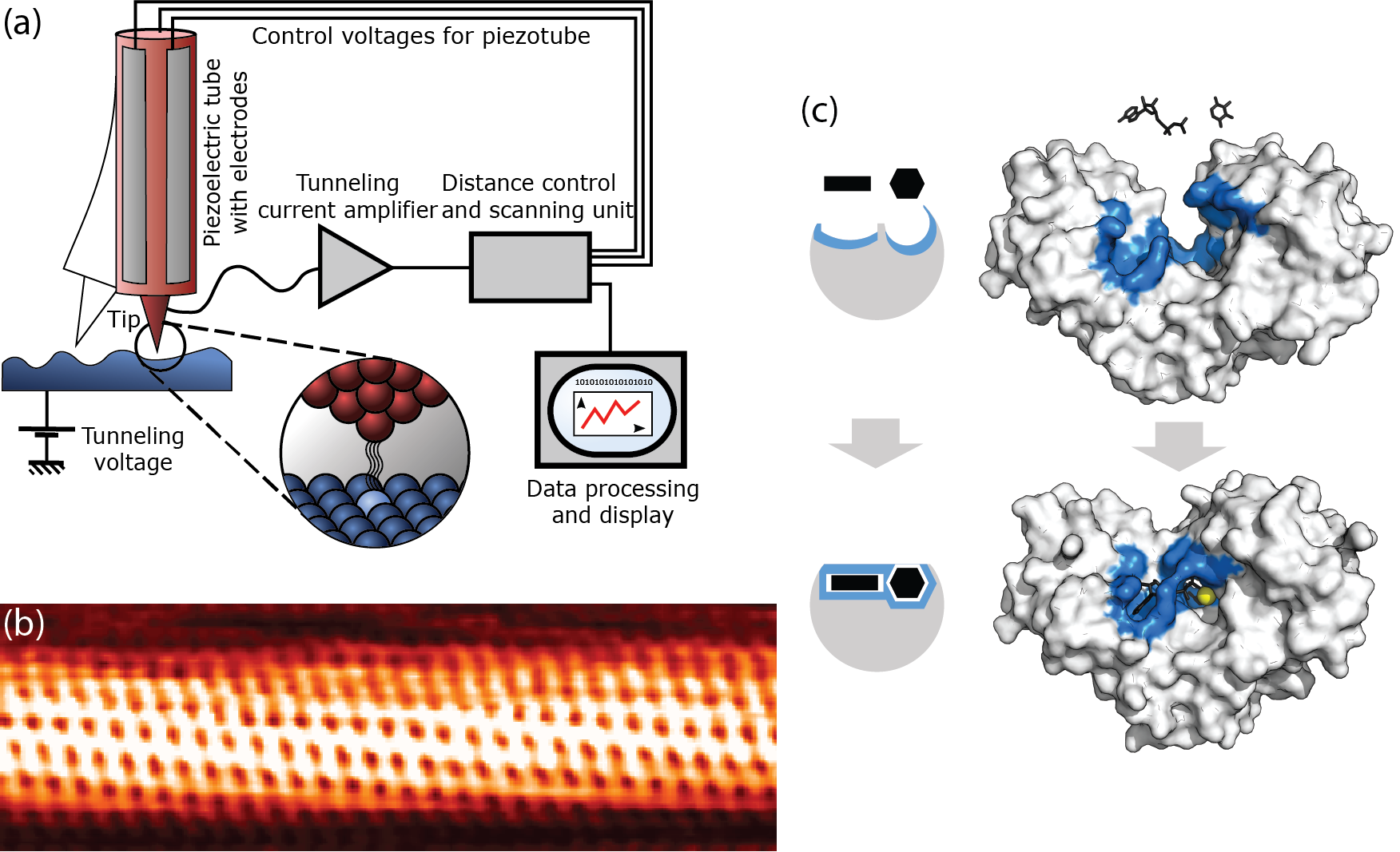
Fig. 2.3 Two applications of tunneling. (a/b) In a scanning tunneling microscope, surfaces can be resolved at atomic length scales by bringing a sharp tip close to the surface, applying a potential difference between the surface and tip, and measuring the resulting tunneling current. (a) Illustration of the method [5]. (b) An atomically resolved image of a carbon nanotube [6]. (c) Biological enzymes catalyze many reactions in the cell. They do so highly specifically by only binding to the exact reagants. The binding typically induces a conformational change in the enzyme, bringing the reagants closer together. In many enzymatic reactions, the reagants exchange either an electron (redox reaction) or a proton (acid-base reaction). The exchange of the electron or proton can be highly accelerated through quantum tunneling, facilitated by a metal ion (which reduces the barrier) in the enzyme. The tunneling rate is measured to be a factor 1000 higher than the reaction rate would be in the absence of quantum effects, making tunneling crucial to many biological processes. The illustration shows how the hexokinase enzyme facilitates the reaction between xylose and adenosine triphosphate (ATP); the yellow spot is a magnesium ion (\(\mathrm{Mg}^{2+}\)) [7].#
Quantum tunneling has many applications in research, technology, and biology. Two examples are illustrated in Fig. 2.3. Tunneling is the basis of the scanning tunneling microscope (STM). In an STM, a (very!) sharp tip is brought in close proximity to a conducting surface. By applying an electric potential across the surface and the tip, a charge difference builds up between them, as in a classical capacitor. Electrons can then tunnel from the tip to the surface, generating a measurable current. Because the distance between the tip and the surface depends on the structure of the surface (it is smaller when the tip is directly above an atom, and larger when it is in between atoms), the current will change as we move the tip, allowing us to re-construct the shape of the surface. An example of such a reconstruction of the surface of a carbon nanotube is shown in Fig. 2.3(b). Tunneling also plays a crucial role in enzymatic reactions in biology, as illustrated in Fig. 2.3(c). Reagants binding to an enzyme commonly induce a conformational change in the enzyme, which not only brings the reagants themselves closer together, but also puts them close to a catalyst in the enzyme, usually one or two metal ions. These metal ions significantly lower the tunneling barrier for the exchange of electrons [Dev80, MS85] or (to a lesser degree, because they are heavier) protons [KK13, SS02] between the reagants. Without the tunneling effect, enzymatic reactions would proceed much more slowly, if at all.
2.2.4. Harmonic potential#
The examples we discussed so far are extremes that couple (relative) mathematical simplicity to lack of physical realism. There are no infinite deep wells or infinitely thin but infinitely high barriers. Even a completely free particle does not exist, and if it would, it would be infinitely boring (as it would be the only thing in the universe). Of course, in many cases you can approximate the actual physics with the crude models of the previous sections, but as soon as you start dealing with actual forces, they fail utterly.
The simplest nontrivial force law in classical mechanics is Hooke’s law, which states that the force exerted by a spring is proportional to the extension of the spring. Consequently, a particle with mass \(m\) suspended on a spring with spring constant \(k\) will oscillate with frequency \(\omega = \sqrt{k/m}\). Spring forces are conservative (i.e., don’t dissipate mechanical energy) and can thus be written as (minus) the derivative of a potential; for a Hookean spring, the potential is given by
In everyday life, many things oscillate, often annoyingly; take, for example, the lid of a pan that you leave upside-down on the kitchen counter. There is no spring attached to the lid; its oscillation can however be understood through the same physics, as close to the minimum of the lid’s potential energy, it can be expanded in a Taylor series, of which the first nontrivial term has the same mathematical form as the harmonic potential in equation (2.41). The same concept holds for quantum potentials: close to a minimum, the Taylor expansion locally closely matches a harmonic potential, and therefore local solutions to the Schrödinger equation will also closely match those of the harmonic potential, at least for the lowest eigenvalues. Note that these solutions will not be oscillations in the classical sense, but rather in the same sense as those we found in the infinite square well: we get standing-wave solutions for definite energies (though with very different shapes than the simple sines in the infinite well) and oscillating solutions for states that are linear combinations of eigenstates.
There are two ways to solve the Schrödinger equation for the harmonic potential (2.41). One is substituting a series solution (see Section 7.4.5), a technique we will also use in Section 2.3 and you can try for yourself in Exercise 2.12. The other technique is algebraic, which is at the same time simpler (the mathematical operations are easier) and harder (as it involves new concepts). We will also use this technique when discussing angular momentum, and if you continue studying the quantum world, you will run into it again for the creation and annihilation of particles.
To set the stage, we write the time-independent Schrödinger equation with a harmonic potential as
If \(\hat{p}\) and \(\hat{x}\) were numbers (or their actions both were to multiply with a number), we could factor the Hamiltonian, writing the term in square brackets as \((p + i m \omega x)(p - i m \omega x)\). Unfortunately, life isn’t that easy with operators, because, as we’ve seen in Section 1.5, the order in which you apply them generally matters, in particular for the position and momentum operators. However, nobody stops us from defining new operators that are combinations of the momentum and position operator, so, inspired by the possibility of factorization, we define[8]
Our two new operators don’t commute; using \([\hat{x}, \hat{p}] = i \hbar\) from equation (1.64), we find
where we used that any operator commutes with itself. By equation (2.44), the operators don’t commute, but the price for switching them is relatively mild, a numerical factor, which comes out at \(-1\) by our choice of the prefactor in the definition of \(\hat{a}_\pm\). Therefore, we can hope to express the Hamiltonian in terms of our new operators, which indeed we can do. To see how, simply apply both operators to the wave function \(\psi(x)\), which gives:
For the Hamiltonian, we can thus write
As it turns out, the ‘almost-factorization’ of equation (2.46) is good enough, because we can use it to construct all the solutions of the Schrödinger equation (2.42). To see how this works, first assume that we have a solution in the form of an eigenfunction \(\psi(x)\) with eigenvalue \(E\). Then the function \(\hat{a}_+ \psi(x)\) is also a solution, with eigenvalue \(E + \hbar \omega\):
Similarly, we find that \(\hat{a}_- \psi(x)\) is a solution with eigenvalue \(E - \hbar \omega\). From a solution \(\psi(x)\) we can thus construct a whole family of solutions by repeatedly applying the operators \(\hat{a}_\pm\). Because these operators effectively increase and decrease the eigenvalue of the solution, they are known as the raising and lowering operators; the family of solutions is sometimes called a ‘ladder’ because they are evenly spaced by \(\hbar \omega\).
We’re not done yet; notwithstanding our nice creation of a whole family of solutions, we do not yet know if any solutions exist, nor if all possible solutions can be constructed from any given one (there could be multiple independent starting points). As it turns out, there is only one family. To see why, consider what happens when we repeatedly apply the lowering operator \(\hat{a}_-\): the energy of the new state is \(\hbar \omega\) lower than that of the previous state. Mathematically that’s fine, but physically we run into trouble at some point: the energy of the particle cannot be less than the minimum of the potential energy. Our potential nicely has its minimum at zero, so the energies always need to be non-negative. Let \(\psi_0(x)\) be the solution with the lowest non-negative solution. Applying \(\hat{a}_-\) would give us a solution with negative energy, unless it returns zero, which is a solution of the Schrödinger equation but not normalizable (and thus not a physical solution). We can thus determine \(\psi_0(x)\) from the condition that \(\hat{a}_- \psi_0(x) = 0\), which gives
Equation (2.48) is a first-order differential equation, which we can solve by separating variables and integrating; the (normalized) solution (see Exercise 2.9) is
Note that, like for the infinite square well, the lowest-energy (ground state) solution has an energy larger than the minimum of the potential: any quantum particle in a harmonic potential will always be moving. Now that we have one solution (which we know to be the unique lowest-energy solution), we can simply construct the whole family of solutions by repeatedly applying the raising operator \(\hat{a}_+\), which gives
Unlike in the case of the infinite well (or the hydrogen atom in Section 2.3), we label the ground state with \(n=0\) for the harmonic oscillator (an unfortunate historical convention). The excited states have positive integer values of \(n\). Expressions for these states can in principle be found using equation (2.50), though going up to \(\psi_{10}\) this way would be rather tedious. Moreover, we would still need to normalize each state (though, as we’ll see, we can get the normalization constant algebraically). In contrast, we get all eigenvalues ‘for free’ without the need of additional calculation. What’s more, we can find the expectation value of many observables without having to obtain explicit expressions for the states \(\psi_n(x)\).
The first step to finding the normalization constants and expectation values is to observe that we can find the value of \(n\) by applying the first the lowering and then the raising operator to any state \(\psi_n(x)\):
where we used equation (2.45)a to re-write \(\hat{a}_+ \hat{a}_-\) in terms of the Hamiltonian, and equation (2.50) to evaluate \(\hat{H} \psi_n(x)\). We can thus define a new operator, the number operator \(\hat{n} = \hat{a}_+ \hat{a}_-\), whose action on \(\psi_n(x)\) returns the value of \(n\): \(\hat{n} \psi_n(x) = n \psi_n(x)\). Likewise, we can show that \(\hat{a}_- \hat{a}_+ \psi_n(x) = (n+1) \psi_n(x)\). Step two is to observe that \(\hat{a}_+\) and \(\hat{a}_-\) are each other’s Hermitian conjugate (see Section 1.4.2 and Exercise 2.10), i.e.
for any two functions \(f(x)\) and \(g(x)\) in our Hilbert space. Combining equations (2.51) and (2.52), we get
Therefore, we get \(\psi_{n+1}(x) = \frac{1}{\sqrt{(n+1)}} \hat{a}_+ \psi_n(x)\). The normalization constant \(A_n\) of the \(n\)-th wave function is thus \(A_n = 1/\sqrt{n!}\). Third, we have that the eigenfunctions of the harmonic oscillator Hamiltonian are orthonormal:
so either \(m=n\) or \(\Braket{\psi_m | \psi_n} = 0\).
To find the expectation value of an observable, remember that all observables are functions of \(\hat{x}\) and \(\hat{p}\). We can express both in terms of our operators \(\hat{a}_\pm\) by inverting equation (2.43):
As an example on how to use these expressions to efficiently calculate the expectation value of an observable for a particle in a state \(\psi_n(x)\), let us consider the potential energy \(V(x)\), which we can express in terms of \(\hat{a}_\pm\) as
For the expectation value of \(V\) we then get
In the third line, we used that \(\hat{a}_+^2 \psi_n \propto \psi_{n+2}\), \(\hat{a}_-^2 \psi_n \propto \psi_{n-2}\), and the fact that the eigenfunctions are orthogonal; we also used equation (2.51) to evaluate the remaining two terms. We find that the expectation value of the potential energy in the \(n\)th state is exactly half the total energy in that state; that’s a specific result for the harmonic oscillator potential that does not generalize to other cases.
2.3. The hydrogen atom#
2.3.1. The Schrödinger equation in three dimensions#
In Section 2.2, we solved the Schrödinger equation for some one-dimensional examples. These examples have the advantage of mathematical simplicity, with solutions of the form of simple sines or Gaussians, but the distinct downside of being physically unrealistic. In classical mechanics, we may, on occasion, be able to restrict a system to one or two spatial dimensions, but in quantum mechanics this turns out to be very complicated. The examples in Section 2.2 thus mostly serve to develop some physical intuition about the quantum world, rather than provide testable predictions. In this section, we’ll study the simplest nontrivial three-dimensional case: that of the wave function and energies of an electron in a hydrogen atom (we’ll take the nucleus, a single proton, which is about 2000 times heavier than the electron, as stationary). This case is realistic and leads to directly testable predictions, but at the same time is at the very limit of our analytical capabilities. Even the next-simplest cases, either the helium atom or molecular hydrogen, have not been solved analytically in closed form, though of course we have techniques of approximating the solutions (we’ll study those in Chapter 5), and we can find them numerically.
To study hydrogen, the first thing we need to do is to generalize the Schrödinger equation to three dimensions. Fortunately, doing so is straightforward: the second derivative in the kinetic energy term becomes a Laplacian, and the potential simply becomes a (still scalar) function of three coordinates:
As long as the potential remains independent of time, the time dependence in the three-dimensional equation is exactly the same as in the one-dimensional case, so we also retrieve the same time-independent form of the Schrödinger equation, \(\hat{H} \psi(\bm{r}) = E \psi(\bm{r})\).
2.3.2. Spherical harmonics#
In our example of interest, the hydrogen atom, the potential is a function of the radial coordinate only[9], so \(V(\bm{r}) = V(r)\). We can then solve equation (2.58) by separation of variables again, splitting it into a radial and an angular part. In spherical coordinates, we write \(\psi(\bm{r}) = R(r) Y(\theta, \phi)\), and (looking up the correct expression for the Laplacian in spherical coordinates), we have
If we now multiply by \(2mr^2/\hbar^2\) and divide through by \(RY\), we find
By the usual argument in separation of variables, as the left-hand side of equation (2.60) depends only on \(r\) (and is thus the same for any value of \(\theta\) or \(\phi\)), and the right-hand side is a function of \(\theta\) and \(\phi\) alone (and thus invariant when changing \(r\)), the only option is that both sides are equal to a (presently arbitrary) constant. For later purposes, we write that constant as \(l(l+1)\).
The angular part of the equation is now independent of the potential, and equal to the angular part of the Poisson equation from electrostatics, \(\nabla^2 \psi = \rho_\mathrm{e}/\varepsilon_0\) (where \(\psi\) is the electrical potential, \(\rho_\mathrm{e}\) the electric charge, and \(\varepsilon_0\) the permittivity of vacuum). Unsurprisingly, the solutions are also the same. They are known as the spherical harmonics, in essence the Fourier components of an expansion in spherical modes, similar to the sines and cosines for a linear expansion. To find the functional form of these spherical harmonics, we split the angular equation again, writing \(Y(\theta, \phi) = \Theta(\theta) \Phi(\phi)\), and substitute into the condition that the right-hand side of equation (2.60) equals \(l(l+1)\). Separating \(\Theta\) and \(\Phi\) then gives:
In equation (2.61), we multiplied both sides with \(\sin^2\theta\) and divided through by \(\Theta \Phi\) to separate the variables. Repeating the same argument as above, both sides have to be equal to a constant, which (again for future purposes) we write as[10] \(m_l^2\). The equation for \(\Phi\) is now easy:
with solutions
Here \(m_l\) can be either positive or negative. As the variable \(\phi\) ‘wraps around the sphere’, \(\Phi(\phi)\) has to be periodic: \(\Phi(\phi) = \Phi(\phi + 2\pi)\), which restricts the possible values of \(m_l\) to integers, and we have \(m_l \in \mathbb{Z}\). These solutions will perhaps not surprise you: we stated above that the spherical harmonics are like the Fourier modes of the sphere, and in the azimuthal (i.e., \(\phi\)) direction, they turn out to be the familiar sines and cosines.
In the polar (i.e., \(\theta\)) direction, things are less easy, as the polar angle runs only from \(0\) to \(\pi\). Our equation for \(\Theta\) reads:
For \(m_l = 0\), the solutions to equation (2.64) can be found through series substitution, which can be done most easily if you first make a coordinate transform from \(\theta\) to \(x = \cos\theta\). The series substitution then gives solutions in the form of the Legendre polynomials \(P_l(x)\), which can most easily be found from the Rodrigues’ formula (see Exercise 2.14):
for any non-negative integer value of \(l\) (i.e., \(l= 0, 1, 2, 3, \ldots\)). Solutions for nonzero \(m_l\) are then derivatives of the Legendre polynomials, known as the associated Legendre polynomials:
Although \(P_l^m(x)\) is defined for any integer value of \(m\), it is identically zero if \(|m|>l\), restricting the number of allowed azimuthal modes. For the polar functions we thus find \(\Theta(\theta) = A P_l^m(\cos\theta)\), and for the spherical harmonics, after normalization[11],
where \(\varepsilon = 1\) if \(m \leq 0\) and \(\varepsilon = (-1)^m\) if \(m>0\). We can rewrite the complex spherical harmonics given here as real functions by making linear combinations, giving sine and cosine dependencies on \(\phi\) rather than complex exponentials. The resulting functions for the first four values of \(l\) are plotted in Fig. 2.4.
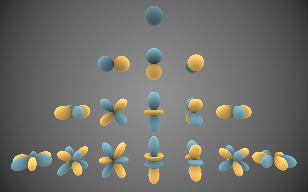
Fig. 2.4 Visual representation of the (real) spherical harmonics for \(l=0, 1, 2, 3\) (top to bottom) [12]. The real harmonics are obtained from the complex ones by linear combinations of \(P_l^m\) and \(P_l^{-m}\), which give sine and cosine functions of \(\phi\), instead of complex exponentials. Blue and yellow shaded regions have opposite sign. The single \(l=0\) harmonic corresponds to uniform expansion / contraction, the three \(l=1\) harmonics to translations in the \(x\), \(y\) and \(z\) directions. Note that the \(m_l = 0\) harmonics (central axis) are always axisymmetric (i.e., invariant under rotations about the \(z\)-axis), and that you can always go from a solution with a positive value of \(m_l\) to one with a negative value by a rotation about the \(z\)-axis over an angle \(\pi / 2m_l\).#
2.3.3. The radial equation#
The spherical harmonics are the solutions of the angular half of equation (2.60). The other half is a function of the radial coordinate \(r\) alone:
In this form, the radial equation is a rather tough nut to crack, as its coefficients are functions of \(r\). Moreover, it contains both a first and a second derivative of \(R(r)\). The term with the first derivative can be removed by introducing a new function, \(u(r) = r R(r)\), which is simply a re-scaling of \(R(r)\). In terms of \(u(r)\), the equation reads
which is similar in form to the one-dimensional Schrödinger equation. The price of the rescaling is that we pick up an extra term in the potential, of the form \(1/r^2\). Something similar happens in classical mechanics when you make a transformation from a fixed to a co-rotating coordinate system: you pick up terms that act like forces on your system. These additional forces are known as ‘fictitious forces’ (as they are not due to a potential but to your choice of coordinates), but their effects are very real [Ide18]. Examples include the centrifugal force and the Coriolis force. The \(1/r^2\) term we have here is a centrifugal term. In a classical picture, the corresponding outward force would compensate the inward Coulomb force on the electron, keeping it in a closed orbit.
Equation (2.69) may look somewhat nicer than (2.68), but it still is a nontrivial eigenvalue problem. We can solve it in two ways: by series substitution and by the use of raising and lowering operators. We’ll work out both, but first we need to ‘rephrase’ the normalization condition in terms of \(u(r)\), as our final solutions will have to be normalized. We have
where we used in the third line that the spherical harmonics are normalized independently. The normalization condition on \(u(r)\) is thus that its square integrates to \(1\) over the range of positive real numbers \(r\).
For the hydrogen atom, we have
We have a continuum of scattering states with \(E>0\), and a discrete spectrum of bound states with \(E<0\). We will solve here for the latter. To simplify the notation, we rescale the energy by dividing equation (2.69) through by \(\hbar^2/2m_\mathrm{e}\), like we did before for the particle in the infinite well, and define:
Note that for bound states, \(\kappa\) is real as \(E\) is negative. I’ve added a subscript ‘e’ to the mass to indicate that we are dealing with the electron mass, and to distinguish from the number \(m_l\). Note that \(\kappa\) has dimensions of length, while \(u\) is dimensionless. If we now divide equation (2.69) by \(\kappa^2\), we get terms that are all dimensionless:
The combination of factors in front of the \(1/r\) term in the square brackets must have dimensions of inverse length, so we can define a characteristic length scale of the hydrogen atom, known as the Bohr radius:
where the choice of taking a numerical factor \(4\) is historical (see equation (1.5)), but will make this length close to (the best definition of) the actual radius, as we will see. The numerical value of the Bohr radius is \(5.29 \cdot 10^{-11}\;\mathrm{m}\), or about half an Ångström. We’ll see that \(\kappa\) and \(a_0\) are closely related.
Finally, we can express the radial coordinate in terms of the length scale \(\kappa\), defining \(\rho = \kappa r\) and \(\rho_0 = 2 / \kappa a_0\). In terms of these rescaled variables, equation (2.73) becomes
We could try a series solution for equation (2.75), but the smarter approach is to check the asymptotic behavior first. In the limit of large \(\rho\), only the first term in parentheses on the right-hand side of equation (2.75) remains, and we are left with an equation that we can easily solve exactly, giving \(u(\rho) = A e^{-\rho} + B e^\rho\). The second term of this solution diverges, and thus cannot be normalized, so we must set \(B=0\); unsurprisingly the radial wave function will drop off like \(e^{-\rho}\) at large values. In the limit that \(\rho \to 0\), we find that the \(1/\rho^2\) term dominates equation (2.75), and again we can solve the equation exactly if we ignore the other two terms, which gives \(u(\rho) = C \rho^{l+1} + D \rho^{-l}\). As negative powers diverge when we approach zero, the second term again cannot be normalized, and we find that \(u(\rho)\) scales as \(\rho^{l+1}\) close to zero. An educated guess for the solution of equation (2.75) would therefore be a function that interpolates between the two limit solutions. Introducing a new function \(v(\rho)\), we write our trial solution as \(u(\rho) = e^{-\rho} \rho^{l+1} v(\rho)\). We then find
At first glance, it seems that we made matters significantly worse: while in equation (2.75) we had gotten rid of the first derivative term through re-scaling, we got it back in (2.76). On the other hand, the asymptotic factors \(e^{-\rho}\) and \(\rho^l\) appear on both sides of the equation and thus drop out, and we can therefore expect \(v(\rho)\) to be well-behaved enough to allow for a series solution. Rearranging terms, our equation now reads:
for which we try a series expansion
where in the second equality of (2.78)b we shifted the summation by one (which we can do as the \(j=0\) term was identically zero). We do not need such a shift in (2.78)c as the second derivative of \(v(\rho)\) is multiplied by \(\rho\) in equation (2.77). Substituting back and collecting like terms, we get
Now for the series to vanish, each individual term must vanish, which gives us a recursion relation between the coefficients:
Given a starting value \(c_0\), we can then find all the \(c_j\)’s. Typically, series solutions come in two flavors: those for which the series terminates at some point (with polynomials as solutions) and those which go on with nonzero terms indefinitely. In this case, the non-terminating series cannot be normalized. To see why, consider the limit in which \(j\) gets large, then (2.80) goes to
The sum of the series with these coefficients is well known: it’s \(e^{2\rho}\). Even with the \(e^{-\rho}\) factor that we will multiply \(v(\rho)\) with to get the full solution, this series diverges at large \(\rho\), and thus will not give us normalizable solutions. The only allowable solutions are thus the ones for which the series terminates at some point, i.e., \(c_{j+1} = 0\) for some value of \(j\). If \(j_\mathrm{max}\) is the largest value of \(j\) for which \(c_j\) is nonzero, we have
so we find that the values of \(\rho_0\) are quantized. The smallest possible value of \(n\) is \(1\) (for \(j_\mathrm{max} = l = 0\)), and \(n\) can take any integer value greater than zero. However, for a given value of \(n\), \(l\) is now restricted from above to \(n-1\), as for a larger value equation (2.82) cannot be satisfied for any nonnegative \(j_\mathrm{max}\).
To get the actual energies, we simply re-substitute the definitions of \(\rho_0\) and \(\kappa\), which gives:
We have retrieved Bohr’s result from Section 1.2.2 (equation (1.6)). That means that we also retrieve the predictions for the absorption and emission spectra of the hydrogen atom. However, the classical orbits Bohr assumed are replaced with wave functions (sometimes referred to as ‘orbitals’), the square of which represents a probability distribution, not a trajectory through space. A measurement of an electron in a state with \(n=2\) might give a position closer to the nucleus than the measurement of an election in the \(n=1\) state. Moreover, the positions are not restricted to a plane, but rather have a spherical symmetry around the nucleus, making them very different from the Keplerian orbits of planets around the sun.
The actual polynomial functions \(v(\rho)\) that are the solutions of equation (2.77) are given in terms of the (associated) Laguerre polynomials \(L_q^p(x)\), defined by
Given values of \(n\) and \(l\), the function \(v(\rho)\) is given by
Substituting back, we can eventually work out the radial function \(R(r)\), which we characterize by \(n\) and \(l\). The (normalized) first six are given by
The radial wave functions are plotted in Fig. 2.5. Note the patterns: the \(l=0\) functions contain a exponential decay with \(l\) crossings of the horizontal axis, while the \(l>0\) functions start at \(0\) and have a well-defined local maximum. The product of these radial functions with the spherical harmonic functions \(Y_l^m(\theta, \phi)\) for the angular part gives the full solution \(\psi_{nlm}(r, \theta, \phi)\). The full wave functions are thus characterized by the three quantum numbers \(n\), \(l\) and \(m_l\), known as the principal, orbital, and magnetic quantum number, respectively[13]. It is an easy exercise to show that for a given value of the principal quantum number \(n\), there are \(n^2\) states. As the energy depends on \(n\) alone, these states will thus be \(n^2\)-fold degenerate.

Fig. 2.5 Radial part of the first six eigenfunctions of the hydrogen Hamiltonian.#
2.4. Problems#
Exercise 2.1 (Linear combinations of stationary states)
Consider the stationary wave functions \(\psi_1(x)\) and \(\psi_2(x)\). Assume that they are normalized solutions to the stationary Schrödinger equation with energies \(E_1\) and \(E_2\) respectively. Now let
be a linear combination of both solutions, with \(c_1\) and \(c_2\) (complex and nonzero) constants. Furthermore assume that \(c_1\) and \(c_2\) are chosen such that \(\Psi\) is normalized.
Show that \(\Psi(x,t)\) is a solution to the time-dependent Schrödinger equation.
Compute the probability density \(|\Psi(x,t)|^2\). Does it depend on \(t\)? In which case is \(\psi = c_1 \psi_1(x) + c_2 \psi_2(x)\) also a solution to the stationary Schrödinger equation?
Show that \(E_1\) (and by similarity also \(E_2\)) must be real. Hint: Write \(E_1 = E + i \Gamma\) with \(E\) and \(\Gamma\) real and show that for \(\Psi_1(x,t) = \psi_1(x)e^{-iE_1t/\hbar}\) to be normalizable for all \(t\) we must have \(\Gamma = 0\).
Show that \(\frac12 (\psi_1 + \psi_1^*)\) is also a solution to the stationary Schrödinger equation. What can you conclude from this observation?
Exercise 2.2 (A particle in an infinite square well)
We consider a particle in the infinite square well, i.e. the potential is given by
where \(a>0\) is a real constant. Let the initial state of the particle (with mass \(m\)) be given by
Find \(A\) such that \(\Psi(x,0)\) is normalized. Hint: this can be done without explicitly computing any integrals.
Find \(\Psi(x,t)\) and compute \(|\Psi(x,t)|^2\) explicitly. Simplify your answer by setting \(\omega = \frac{\pi^2 \hbar }{2ma^2}\).
Compute \(\Braket{\hat{x}}\). Does it depend on time? Why (not)?
Compute \(\Braket{\hat{H}}\).
If an energy measurement is performed on \(\Psi(x,t)\) at time \(t\), what outcomes can we get and with what probability? Is \(\Braket{\hat{H}}\) a possible outcome? Why (not)?
Exercise 2.3 (Particle phase in the infinite square well)
We consider a particle in the infinite square well, i.e. the potential is given by
where \(a>0\) is a real constant. Let the initial state of the particle (with mass \(m\)) be given by
where \(0 \leq \phi < 2 \pi\) is an arbitrary phase and \(\psi_1\) and \(\psi_2\) are the first two eigenstates of the Hamiltonian.
Find \(\Psi(x,t)\) and \(|\Psi(x,t)|^2\) in terms of \(\psi_1\), \(\psi_2\), \(E_1\), \(E_2\) and \(\phi\).
Find \(\Braket{\hat{x}}\) and \(\Braket{\hat{p}}\). Do they depend on time? What is the role of \(\phi\)? Use \(\omega = \frac{\pi^2 \hbar}{2ma^2}\) to simplify the result. Hint: Use Ehrenfest’s theorem to relate \(\Braket{\hat{x}}\) and \(\Braket{\hat{p}}\) through a classical law.
What energies can be obtained if a measurement is performed? With what probabilities? Also, find \(\braket{\hat{H}}\).
Suppose now that at \(t=0\) the well suddenly expands and the right wall is moved to \(x = 2a\). The initial wave function is unchanged by this process.
What are now the four smallest outcomes an energy measurement could yield? What are the probabilities of finding them? To simplify the calculation you may set \(\phi = 0\) here.
Find \(\braket{\hat{H}}\) again.
Exercise 2.4 (A free particle)
Suppose we have a particle of mass \(m\) in the initial state
where \(A\) and \(a\) are real and positive constants.
Normalize the wave function.
For what potential is the initial state a stationary state? Is it the ground state of this potential? What is the corresponding energy?
Find \(\braket{\hat{H}}\) at \(t=0\), using the general method
Is this in agreement with your previous answer?
Now we assume that we have the initial state \(\Psi(x,0)\) in a zero potential. Find \(\phi(k)\), the Fourier transform of the initial wave function. Hint: You can solve the integral by hand if you use integration by parts twice.
Find \(\Psi(x,t)\) in terms of an integral over the wavenumber \(k\).
Exercise 2.5 (Gaussian wave packet)
We consider a free particle with a wave function initialized as
where \(a\) and \(A\) are real, positive constants.
Normalize \(\Psi(x, 0)\), i.e., find \(A\).
Find \(\phi(k)\), i.e. the weight of the eigenstate with wavenumber \(k\) (cf. equation (2.28)).
Show that the time evolution of the particle’s wave function is given by
(2.89)#\[\Psi(x, t) = \frac{A}{\sqrt{\gamma}} e^{-a x^2 / \gamma},\]where \(\gamma\) is a number that depends on time. Find an expression for \(\gamma\).
Find \(|\Psi(x, t)|^2\) and sketch it for \(t=0\) and some large value of \(t\). Hint: it will help to group some numbers together.
Exercise 2.6 (Bound state of the Dirac delta potential)
In this problem, we’ll find the bound state of the Dirac delta potential well (and prove that there is only one). Our potential is the same as in equation (2.31), with the restriction that \(\varepsilon < 0\) (as for positive values of \(\varepsilon\) we have a barrier, not a well, and hence no bound states). The time-independent Schrödinger equation then reads:
As we’re looking for bound states, we want solutions with \(E<0\).
As \(E<0\), we can define the (real, positive) number \(\kappa = \sqrt{-2mE}/\hbar\). Re-write equation (2.90) in terms of \(\kappa\).
Find the general solution to (2.90) for \(x<0\).
Also find the general solution to (2.90) for \(x>0\).
Of the solutions in (b) and (c), cross out the ones that diverge.
Apply the condition that \(\psi(x)\) be continuous at \(x=0\) to eliminate one of the constants in your solutions.
Apply the condition (2.36) on the derivative of \(\psi(x)\) to find the allowed value of \(\kappa\), and hence of \(E\).
Normalize the solution.
Plot the wavefunction and the probability density.
Exercise 2.7 (The double delta potential)
In this problem we will consider the symmetric double delta potential well, given by
where \(\alpha\) is a positive constant of appropriate dimension (Joule \(\times\) meter, such that the potential is in Joule). This potential function is even (i.e. \(V(x) = V(-x)\)) and therefore the bound state solutions are either even (\(\psi_\mathrm{even}(x) = \psi_\mathrm{even}(-x)\)) or odd (\(\psi_\mathrm{odd}(x) = - \psi_\mathrm{odd}(-x)\)). Since we are looking for a bound state, we have \(E < 0\). Define \(\kappa = \frac{\sqrt{-2mE}}{\hbar} > 0\).
Write out the general form of the even solution using constants complex \(A\) and \(B\), \(\kappa\) and exponentials. Exploit the symmetry of the solution.
Impose the continuity of \(\psi\) and the appropriate discontinuity of its derivative at \(x=a\). Use these two equations to eliminate the complex constants \(A\) and \(B\). Find the equation that relates the unknown \(\kappa\) to other known physical constants (including \(\alpha\) and \(a\)).
How many solutions does this equation have? What does this mean?
Proceed in the same way (questions b-d) for finding the odd solution(s).
Exercise 2.8 (An infinite square well with an internal barrier)
In this problem, we consider the infinite square well potential with an internal barrier. To be able to exploit the symmetry of the system, we’ll shift the well such that it is centered around zero, and the potential reads
For energies much larger than \(V_0\), the eigenstates of the Hamiltonian corresponding to this potential will essentially be the same as those for an infinite well. For energies smaller than \(V_0\) however, the region \(-a < x < a\) will be classically forbidden. We did not solve the Schrödinger equation for such a finite barrier in class, but the solution method is straightforward, as the potential is piecewise constant. The pieces can then be glued together by the boundary condition that the wavefunction and its derivative must be continuous at \(x=a\). Unfortunately, these conditions give us equations that we cannot solve analytically, and thus we are reduced to numerical methods. Those methods tell us that there are two solutions with energies very close together: the ground state, which is symmetric (or ‘even’, like the cosine) and the first excited state which is antisymmetric (or ‘odd’, like the sine). We call the ground state \(\psi_\mathrm{e}\) with energy \(E_\mathrm{e}\), and the excited state \(\psi_\mathrm{o}\) with energy \(E_\mathrm{o}\). They are plotted in Fig. 2.6 on top of a sketch of the potential itself.

Fig. 2.6 The infinite square well potential with an internal barrier (equation (2.91)) in dashed gray, with the (even) ground state \(\psi_\mathrm{e}\) and (odd) first excited state \(\psi_\mathrm{o}\) plotted on top in blue and (dashed) red.#
As you can see from the plot, for the finite barrier there is a small but nonzero probability of finding the particle inside the classically forbidden region. Moreover, in both states, the particle will, over time, oscillate between being on the left and being on the right of the potential. To see how that comes about, suppose that we prepare a particle such that it is initially in a linear combination of the two states, given by
A particle in the \(\psi_+\) linear combination will almost certainly be on the right of the barrier, and a particle in the \(\psi_-\) combination will almost certainly be on the left. Suppose at time \(0\) we prepare a particle in the state \(\psi_+\).
Write down the time-dependent wavefunction \(\Psi(x, t)\) for the particle in the initial state \(\psi_+(x)\). Give your answer in terms of \(\psi_\mathrm{e}(x)\), \(\psi_\mathrm{o}(x)\), \(E_\mathrm{e}\) and \(E_\mathrm{o}\).
Show / argue that after a time interval \(\Delta T = \pi \hbar / (E_\mathrm{o}-E_\mathrm{e})\) the particle, initially right of the barrier, has tunneled through it to the left.
As an application of the well-with-barrier potential, we consider the ammonium molecule \(\mathrm{NH}_3\), which consists of one nitrogen and three hydrogen atoms. Because ammonia contains four nuclei and ten electrons, despite its relative simplicity it is already a highly complicated dynamical system. However, we can get quite far by some approximations. One such approximation is treating the covalent bonds formed by the electrons is as if they were springs keeping the nuclei together (this works because the harmonic potential is quadratic, and the expansion of any potential around any minimum will at lowest order have a quadratic term); the nuclei then just oscillate around the equilibrium positions defined by the potential energies of the ‘electron springs’. For ammonia, the equilibrium configuration is attained when the three hydrogen nuclei form an equilateral triangle, with the nitrogen molecule some distance \(z\) above or below the plane of the triangle, defining two possible minima with a barrier in between. To simplify notation, we define \(\ket{\mathrm{e}}\) and \(\ket{\mathrm{o}}\) as the even and odd eigenstates of the corresponding Hamiltonian, with energies \(E_\mathrm{e}\) and \(E_\mathrm{o}\) as before. The \(\ket{+}\) state is then the linear combination in which the nitrogen atom lies (almost certainly) above the plane of the hydrogen triangle, and \(\ket{-}\) the linear combination in which it lies below the plane:
\[\ket{\pm} = \frac{1}{\sqrt{2}} \left( \ket{\mathrm{e}} \pm \ket{\mathrm{o}}\right).\]Find the matrix elements \(\braket{+|\hat{H}|+}\), \(\braket{+|\hat{H}|-}\), and \(\braket{-|\hat{H}|-}\) in terms of the energies \(E_\mathrm{e}\) and \(E_\mathrm{o}\). Hint: use what you know of the eigenstates of the Hamiltonian, but indicate which properties you use.
Argue that we can represent the Hamiltonian with the following matrix
\[\begin{split}\hat{H} = \begin{pmatrix} \bar{E} & -A \\ -A & \bar{E}, \end{pmatrix}\end{split}\]and find expressions for \(\bar{E}\) and \(A\) in terms of \(E_\mathrm{e}\) and \(E_\mathrm{o}\).
Due to the electronic structure of ammonia, the nitrogen atom carries a small negative charge \(-q\), with a corresponding positive charge \(+q\) distributed among the hydrogen atoms. If the molecule is in either the \(\ket{+}\) or \(\ket{-}\) state, there is a separation of charge, and the molecule therefore become an electric dipole. Because (as you argued in part b), the molecule will oscillate between these two states, it is an oscillating dipole, and thus will emit electromagnetic radiation; it indeed does so at a frequency of \(150\;\mathrm{GHz}\) (i.e., in the microwave range).
From the given frequency of the dipole radiation, find the difference in energy between the ground state (\(E_\mathrm{e}\)) and the first excited state (\(E_\mathrm{o}\)) of ammonia. Express your answer in electronvolts (\(\mathrm{eV}\), one electronvolt is the energy an electron gets when passing through a potential difference of one volt).
Exercise 2.9 (Ground state of the harmonic oscillator)
Through separation of variables and integrating (see Section 7.4.1), solve the first-order differential equation (2.48) for the ground state of the harmonic oscillator potential.
Find the normalization constant of the harmonic oscillator ground state.
Find the energy of the harmonic oscillator ground state. Hint: use equation (2.46) for the Hamiltonian in combination with the defining property of the ground state \(\psi_0(x)\).
Exercise 2.10 (Harmonic oscillator operators)
Prove that the raising and lowering operators \(\hat{a}_\pm\) of the harmonic oscillator potential are each other’s Hermitian conjugates, i.e., that equation (2.52) holds.
Exercise 2.11 (Combining harmonic oscillator states)
As we’ve seen in Section 2.2.4, we can find the eigenstates of the one-dimensional harmonic potential, \(V(x) = \frac12 m \omega^2 x^2\), through repeated application of the raising operator \(\hat{a}_{+}\) on the ground state \(\psi_0(x)\), and we get the ground state itself from the condition that acting on it with the lowering operator \(\hat{a}_{+}\) should give zero (i.e., \(\hat{a}_- \psi_0 = 0\)).
Construct and normalize the first excited state, \(\psi_1(x)\), which is proportional to \(\hat{a}_+ \psi_0(x)\). Verify that your result satisfies the general rule that
(2.93)#\[\psi_n = \frac{1}{\sqrt{n!}} \left(\hat{a}_+\right)^n \psi_0(x).\]Construct a new, normalized state \(\psi\), which is a linear combination of \(\psi_0\) and \(\psi_1\), i.e., \(\psi = c_0 \psi_0 + c_1 \psi_1\), such that \(\Braket{\hat{x}}\) is as large as possible. The answer, as you might guess, is given by
(2.94)#\[\psi = \frac{1}{\sqrt{2}} \left( \psi_0(x) + \psi_1(x) \right).\]For a full solution, you’d have to allow the coefficients \(c_0\) and \(c_1\) to take complex values, but for here, it suffices to take them to be real. You may use without needing to prove it that the eigenstates of the harmonic potential Hamiltonian are orthogonal.
A particle is initialized at \(t=0\) in the state \(\psi\) you constructed at (b). Give its time evolution, i.e., give the \(\Psi(x, t)\) corresponding to this wave function \(\Psi\).
If you were to measure the energy of the state, would it matter at which point in time you do so?
Exercise 2.12 (Eigenfunctions of the harmonic oscillator potential)
In Section 2.2.4 we found the eigenvalues of the Hamiltonian with the harmonic oscillator potential. We also found a method to construct the eigenfunctions, by repeatedly acting with the raising operator \(\hat{a}_+\) on the ground state wave function \(\psi_0(x)\). While in many cases we’ll encounter later we’d already be glad to have numbers for the eigenvalues, in this case, we can also solve for the eigenfunctions directly, using a series expansion approach (see Section 7.4.5). The steps we follow here will also be the ones we’ll employ to find the radial part of the eigenfunctions of hydrogen atom in Section 2.3.3.
First, to avoid mistakes due to factors floating around, we’ll rescale our variables to get the equation in the simplest form possible. Introduce \(\xi = \sqrt{m\omega/\hbar} x\) and \(K = 2E/\hbar\omega\), and show that in these variables, the time-independent Schrödinger equation with the harmonic oscillator potential (equation (2.42)) can be written as
(2.95)#\[\frac{\mathrm{d}^2 \psi}{\mathrm{d}\xi^2} = \left(\xi^2 - K \right) \psi.\]Before attempting a series solution, we should look at the asymptotic behavior of the solution. If that turns out to be exponential, we need to factorize the solution first, as otherwise the series will not converge. In the present case, for very large values of \(\xi\) (and equivalently very large values of \(x\)), we have \(\xi^2 \gg K\), so we can approximate equation (2.95) as
(2.96)#\[\frac{\mathrm{d}^2 \psi}{\mathrm{d}\xi^2} = \xi^2 \psi.\]Equation (2.96) suggests an Ansatz of the form \(\psi = \exp(\lambda \xi^2)\). Substitute this Ansatz to get possible values for \(\lambda\). NB: you will not get an exact solution - there will be a remainder term. However, we’re not after the exact solution here, but the asymptotic behavior, which will scale like the Ansatz.
Of the two solutions you found in (b), one is not normalizable (as it diverges as \(x \to \pm \infty\)), so we drop it. Retaining the other term, we try a solution of the form
\[\psi(\xi) = u(\xi) e^{-\frac12 \xi^2}.\]Find the differential equation for \(u(\xi)\).
We now try a power series solution for \(u(\xi)\), i.e., we write \(u(\xi)\) as
(2.97)#\[u(\xi) = \sum_{k=1}^\infty a_k \xi^k.\]Substitute equation (2.97) in your differential equation for \(u(\xi)\), then rearrange terms such that the equation is of the form of a power series (i.e., find the coefficients of \(\xi^k\), see equation (7.78)).
From the power series solution, get a recurrence relation for the coefficients \(a_k\).
There are now two options: either the power series goes on forever, or it truncates at some finite value of \(k\). We’ll first show that the first option gives a non-normalizable solution. From your recurrence relation, you should be able to read off that for large values of \(k\), we approximately have \(a_{k+2} = (2/k)a_k\), with (approximate) solution
(2.98)#\[a_k \approx \frac{A}{(k/2)!},\]with \(A\) a constant. Find the function \(u(\xi)\) for the ‘solution’ (2.98), and argue it won’t be an acceptable solution.
Having ruled out the possibility that the series continue forever, it has to terminate at some point. From that condition, get the possible values of \(K\), and thus of the energy eigenvalue \(E\).
As the recurrence relation only contains \(a_k\) and \(a_{k+2}\), we get two qualitatively distinct sets of solutions, one with all ‘odd-\(k\)’ \(a_k\)’s equal to zero (giving an even function) and one with all ‘even-\(k\)’ \(a_k\)’s equal to zero (giving an odd function). Argue why only one of the two sets is permissable at a given time.
We get the two solutions from initial conditions \(a_1=0\) and \(a_0 = 0\), respectively. The resulting polynomials for \(u(\xi)\) are multiples of the Hermite polynomials, denoted \(H_n(\xi)\). Find \(u(\xi)\) for \(n=0, 1, 2, 3\).
Find \(\psi_0(x)\) and \(\psi_1(x)\).
Exercise 2.13 (The shifted harmonic oscillator)
Consider the one-dimensional harmonic oscillator with a uniform electric field \(\mathcal{E}\) (we use \(\mathcal{E}\) for electric field and reserve \(E\) for energy). The potential energy then becomes \(V(x) = \frac{1}{2} m \omega^2 x^2 - e \mathcal{E} x\), where \(e\) is the electron charge.
Sketch the potential.
Write down the Schrödinger equation for this problem.
Use a coordinate transformation of the form \(z = x - C\), where \(C\) is a constant (possibly depending on \(e\), \(\mathcal{E}\), \(m\), \(\hbar\) or \(\omega\)), to transform the Schrödinger equation of this problem into the equation for the unperturbed harmonic oscillator. What is \(C\)?
What are the eigenfunctions and energies of this problems (let us denote them \(\tilde{\psi}_n\) and \(\tilde{E}_n\)) in terms of \(\psi_n\) and \(E_n\), the eigenfunctions and energies of the unperturbed harmonic oscillator.
For what field strength \(\mathcal{E}\) can we find a ground state with zero energy?
Exercise 2.14 (Spherical harmonics)
In this problem, we find the solution to the \(\theta\)-dependent part of the equation for spherical harmonics, (2.64), using a series expansion.
Our first step is a coordinate transformation. Define \(x = \cos(\theta)\) and \(P(x) = P(\cos(\theta)) = \Theta(\theta)\), and show that in terms of \(x\) and \(P\), equation (2.64) can be written as:
(2.99)#\[\left(1-x^2\right) \frac{\mathrm{d}}{\mathrm{d}x} \left[ \left(1-x^2\right) \frac{\mathrm{d}P}{\mathrm{d}x} \right] + \left[ l(l+1) \left(1-x^2\right) - m_l^2 \right] P(x).\]Setting \(m_l = 0\), we can simplify equation (2.99) (technically if \(x^2 \neq 1\)) and rewrite it as
(2.100)#\[\frac{\mathrm{d}}{\mathrm{d}x} \left[ \left(1-x^2\right) \frac{\mathrm{d}P}{\mathrm{d}x} \right] + l(l+1) P(x) = \left(1-x^2\right) \left(1-x^2\right) \frac{\mathrm{d}^2 P}{\mathrm{d}x^2} - 2 x \frac{\mathrm{d}P}{\mathrm{d}x} + l (l+1) P(x) = 0,\]known as Legendre’s differential equation. We then try a series solution for \(P(x)\) of the form
(2.101)#\[P(x) = \sum_{n=0}^\infty a_n x^n.\]Substitute (2.101) into equation (2.100) and rewrite the resulting equation as a single sum over \(n\).
From the condition that the sum only vanishes if each of its term vanishes, find a recurrence relation for the coefficients \(a_n\).
Show that, for large values of \(n\), the recurrence relation scales like the geometric series, which converges if \(|x| < 1\), but not for \(|x| = 1\). Quick reminder: The geometric series is given by
(2.102)#\[\sum_{n=0}^\infty x^n = \frac{1}{1-x} \quad \text{for} \quad |x|<1.\]As our function should also converge at the boundaries where \(|x|=1\), we conclude that our series must terminate.
From the recurrence relation, argue that there are two independent series solutions to our differential equation (2.100), one with only even and one with only odd terms.
We look for solutions for which \(a_0 \neq 0\), \(a_1 = 0\) and the series terminates. Find the condition on the largest nonzero coefficient \(a_n\) for which these requirements are satisfied. Note: you should get two possibilities, but one will give you an empty series. We have now shown that we can write the solution of equation (2.100) as a finite series, i.e., a polynomial. While we can give an expression for this polynomial, it is rather ugly. Instead, we’d like to work with Rodrigues’ formula, given by equation (2.65). Given the formula, it is straightforward to show that the solutions indeed satisfy Legendre’s equation.
First, find the solution to the Legendre differential equation for \(l=0\), and show that your answer is consistent (up to a normalization factor) with Rodrigues’ formula.
Evaluate the following expression for arbitrary integers \(l > 0\):
(2.103)#\[\left( x^2 - 1 \right) \frac{\mathrm{d}}{\mathrm{d}x} \left( x^2 - 1 \right)^l,\]and rewrite it as \(2 l x \left(x^2-1\right)^l\).
Rearranging the result of (g), and taking another \(l+1\) derivatives, we have:
(2.104)#\[0 = \frac{\mathrm{d}^{l+1}}{\mathrm{d}x^{l+1}} \left[ \left( x^2 - 1 \right) \frac{\mathrm{d}}{\mathrm{d}x} \left( x^2 - 1 \right)^l - 2 l x \left(x^2-1\right)^l \right].\]Rewrite equation (2.104) to show that it is equivalent to
(2.105)#\[0 = \frac{\mathrm{d}}{\mathrm{d}x} \left\lbrace \left( x^2 - 1 \right)^l \frac{\mathrm{d}}{\mathrm{d}x} \left[ \frac{\mathrm{d}^l }{\mathrm{d}x^l} \left( x^2 - 1 \right)^l \right] \right\rbrace + l (l+1) \frac{\mathrm{d}^l }{\mathrm{d}x^l} \left( x^2 - 1 \right).\]From equation (2.105), conclude that the function
(2.106)#\[\frac{\mathrm{d}^l }{\mathrm{d}x^l} \left( x^2 - 1 \right)^l\]satisfies Legendre’s differential equation (2.100), and therefore that Rodrigues’ formula (2.65) indeed gives us solutions to that equation.
Finally, to understand the choice of the prefactor (i.e., normalization) in Rodrigues’ formula, calculate the \(l\)th derivative of the leading term (of order \(2l\)):
(2.107)#\[\frac{\mathrm{d}^l }{\mathrm{d}x^l} x^{2l},\]and conclude that we must choose \(1/(2^l l!)\) as the prefactor to the expression given in equation (2.106) to normalize it on the interval \([-1, 1]\).
Exercise 2.15 (The first excited state of the hydrogen atom)
The radial part of the Hamiltonian of a hydrogen atom (or, strictly speaking, the electron in that atom) is given by
where \(\hbar\) is Planck’s constant, \(m_\mathrm{e}\) and \(e\) the mass and charge of the electron, and \(k\) the proportionality constant from Coulomb’s law. The wave function of hydrogen in the ground state (the \(100\) or \(1s\) state) is radially symmetric and given by
where \(a\) is the Bohr radius.
Prove that \(\psi_{100}(r)\) is indeed an eigenfunction of the Hamiltonian (2.108), and find both the associated energy and the value of the Bohr radius in terms of \(\hbar\), \(m_\mathrm{e}\), \(e\), and \(k\).
The wave function for hydrogen in the \(200\) (or \(2s\)) state is given by
(2.110)#\[\psi_{200}(\bm{r}) = \frac{1}{\sqrt{32\pi a^3}} \left(2 - \frac{r}{a}\right) e^{-r/2a}.\]To calculate probabilities and expectation values of a particle in the \(\psi_{200}\) state requires integrating over three-dimensional space. Fortunately, this state, like the ground state, is radially symmetric: it is independent of the angles \(\theta\) and \(\phi\). For any such radially symmetric function \(f(r)\), we can simplify the volume integral to a one-dimensional integral by switching to spherical coordinates:
(2.111)#\[\int_{\text{all space}} f(r) \,\mathrm{d}V = \int_0^\infty f(r) 4 \pi r^2 \,\mathrm{d}r.\]In this problem, you may use the following integrals:
\[\int_0^1 r^2 e^{-r} \,\mathrm{d}r = 2 - \frac{5}{e}, \qquad \int_0^1 r^3 e^{-r} \,\mathrm{d}r = 6 - \frac{16}{e}, \qquad \int_0^1 r^4 e^{-r} \,\mathrm{d}r = 24 - \frac{65}{e}.\]Find the probability that an electron in the \(200\) state of hydrogen will be found a distance less than \(a\) from the nucleus.
Find the expectation values of \(r\) and \(r^2\) for an electron in the \(200\) state of hydrogen. Express your answers in terms of the Bohr radius \(a\).
An electron in the \(200\) state of hydrogen can transition to the \(100\) state under the emission of a photon. Find the frequency of that photon in terms of \(\hbar\), \(m_\mathrm{e}\), \(e\), and \(k\). Hint: combine your answer to part (a) with what you know about the energies of the eigenstates of hydrogen - this will save you a lengthy calculation!
Exercise 2.16 (Quantum dots)
From Wikipedia: ‘’Quantum dots are tiny semiconductor particles a few nanometres in size, having optical and electronic properties that differ from larger particles due to quantum mechanics. \ldots Quantum dots are sometimes referred to as artificial atoms, emphasizing their singularity, having bound, discrete electronic states, like naturally occurring atoms or molecules.’’ Quantum dots are used frequently in experiments (including biological ones) as probes; there also exist biocomposite quantum dots that can be fabricated by viruses. In this problem, we’ll treat a quantum dot as a spherical cavity: electrons can move around freely inside, but cannot escape. The solutions of the Schrödinger equation then separate like they do for the hydrogen atom: \(\psi_{nlm}(r, \theta, \phi) = R_{nl}(r) Y_l^m (\theta, \phi)\). The angular part is still given by the spherical harmonics, and for the radial part we have
where \(E_{nl}\) is the (energy) eigenvalue of the full function \(\psi_{nlm}\). NB: Note that the \(\psi_{nlm}\) here are not the eigenfunctions of the hydrogen atom. The first step to solving equation (2.112) is to re-scale the energy and position variable, writing \(k = \sqrt{2 \me E_{nl}}/\hbar\) and \(z = kr\).
Show that you can re-write equation (2.112) in terms of \(k\) and the variable \(z\) as
(2.113)#\[\frac{\mathrm{d}^2 R}{\mathrm{d}z^2} + \frac{2}{z} \frac{\mathrm{d}R}{\mathrm{d}z} + \left( 1 - \frac{l(l+1)}{z^2} \right) R = 0.\]The solutions to equation (2.113) are the spherical Bessel functions \(j_l(z)\) and spherical Neumann functions \(n_l(z)\). The first two of each are given by
\[\begin{split}\begin{alignat*}{3} j_0(z) &= \frac{\sin(z)}{z}, & j_1(z) &= \frac{\sin(z)}{z^2} - \frac{\cos(z)}{z}, \\ n_0(z) &= -\frac{\cos(z)}{z}, \qquad & n_1(z) &= -\frac{\cos(z)}{z^2} - \frac{\sin(z)}{z}. \end{alignat*}\end{split}\]Verify that both \(j_0(z)\) and \(n_0(z)\) are indeed solutions to your equation at (a).
By expanding the sine and cosine functions around \(z=0\) (note that \(z\) is a real number here), determine which of the two sets will give physically allowable solutions.
Let \(r=a\) be the radius of the quantum dot, then (obviously) we must set \(R(r=a) = R(z=ka) = 0\). Unfortunately, the radial Bessel and Neumann functions do not have nice regularly spaced zeros. Except for the \(l=0\) case, we can’t even compute the positions of the zeros analytically. Therefore, let \(\gamma_{n,l}\) be the \(n\)th zero of the \(l\)th spherical Bessel/Neumann (we only need one, as we’ve dropped the other) function.
Express the energy \(E_{n,l}\) in terms of \(\gamma_{n,l}\).
Compute the numerical value (in electron volts) of the ground-state energy \(E_{1,0}\) for a quantum dot with a radius of \(1.0\;\mathrm{nm}\).
Find the wavelength of a photon emitted by an electron when transitioning from the \(n=2, l=0\) state tot the \(n=1, l=0\) state of a quantum dot.
Evaluate the probability that an electron in the ground state of a quantum dot will be found inside a sphere of radius \(a/2\).
Exercise 2.17 (The virial theorem)
The virial theorem relates the expectation values of the kinetic energy and the work to each other. In this problem, we’ll prove and apply both the one-dimensional and three-dimensional versions of the theorem.
Using the generalized Ehrenfest theorem (equation (1.74)), show that for a one-dimensional system
(2.114)#\[\frac{\mathrm{d}}{\mathrm{d}t} \Braket{\hat{x} \hat{p}} = 2 \Braket{\hat{K}} - \Braket{x \frac{\mathrm{d}V}{\mathrm{d}x}}.\]In a stationary state, the left-hand side of equation (2.114) vanishes, and therefore
(2.115)#\[2 \Braket{\hat{K}} = \Braket{x \frac{\mathrm{d}V}{\mathrm{d}x}} \equiv \Braket{W},\]where \(W\) is the work (force times displacement). Equation (2.115) is known as the virial theorem; it is the quantum-mechanical equivalent of the work-energy theorem in classical mechanics.
Use the virial theorem to show that \(\Braket{\hat{K}} = \Braket{\hat{V}}\) for stationary states of the harmonic oscillator potential.
Now prove the three-dimensional version of the virial theorem:
Theorem 2.1 (Virial theorem)
For a stationary state, the expectation values of the kinetic and potential energies are related through
(2.116)#\[2 \Braket{\hat{K}} = \Braket{ \bm{r} \cdot \bm{\nabla} V }.\]Apply the virial theorem to the stationary states of the hydrogen atom. Show that for these states we have \(\Braket{\hat{K}} = -E_n\), and therefore \(\Braket{\hat{V}} = 2 E_n\).