
2. Essential background#
2.1. Optics#
2.1.1. Lensmaker’s formula, thin lens approximation#
Microscopes work by virtue of lenses that deflect the incoming radiation and can bring this radiation to a focus on the other side of the lens. An important characteristic of a lens is its focal distance \(f\): the shorter the focal distance, the larger the deflection angle, the stronger the lens. If we use a lens to create an image from an object located on the other side of the lens, the image distance from the lens, \(v\), is related to the object distance, \(u\), via the focal distance in the famous lensmaker’s formula:
The transverse (or geometric) magnification of the lens is given by the ratio between image and object distance:
Besides with the transverse magnification, a lens can also be characterized by the angular magnification, which indicates the change in opening angle of the beam on object versus image plane. The angular magnification is the inverse of the transverse magnification:
These properties can be easily understood by tracing rays on either side of the lens. The below video illustrates the above relations via ray tracing with a single lens plane. This is what we call the thin lens approximation. Note that in practise the thin lens approximation does not hold for the lenses we use in electron microscopes but for the basic understanding we aim for in this course, understanding the thin lens approximation is sufficient.
2.1.2. Aberrations#
2.1.2.1. Spherical aberration#
A perfect lens should focus all incoming parallel rays on one side of the lens into a tight focus on the other side of the lens. This means that the deflection angle imposed by the lens should increase linearly with distance to the optical axis. Also, the deflection should be circularly symmetric, meaning the deflection angle for a rays travelling on opposite positions to the optical axis should of the same magnitude but of opposite sign: both rays should cross in the focal point.
In practise, lenses are never ideal and not all rays cross the optical axis precisely in the focal point. This deviation from ideal behaviour is what we call spherical aberration. Spherical aberration leads to a blurring of the focal spot to a disk of radius \(r_{sph}\). The video explains spherical aberration and derives an expression for \(r_{sph}\) based on lens and incoming beam properties. Note that in electron microscopy, opening angles for the electron beam are typically very small, meaning we use the approximation \(sin(\alpha) = \alpha\) and we express angles in radians as opposed to degrees. To give you an idea, beam opening angles in electron microscopy are typically around \(10 \: mrad\).
We thus see that for a situation with an incoming parallel beam, the radius of spherical aberration is given by
where \(\alpha\) is the opening angle in the image plane and \(C_S(\infty)\) is a lens-specific spherical aberration coefficient. If the lens operates at a finite magnification \(M_T\), the spherical aberration coefficient is given by
2.1.2.2. Chromatic aberration#
Besides aberrations due to lens imperfections, the focus or image may also be aberrated due to the rays travelling at different speed through the lens medium. For light optics, this is due to the illumination light consisting of multiple wavelengths and the fact that the refractive index is wavelength-dependent: \(n = n(\lambda)\). In the case of electron optics, chromatic aberration occurs due to electrons travelling with different velocities, thus due to (kinetic) energy dispersion.
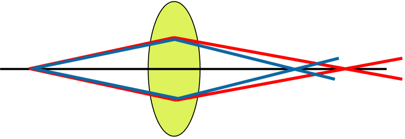
Fig. 2.1 Chromatic aberration: as blue light refracts stronger than red light, at the focal position for the blue light, the red light is blurred. On the other hand, at the red light focus, the blue light is blurred and at the in-between position for least circumference, both colours are defocused.#
Similar to the case of spherical aberration, an expression for the defocus due to chromatic aberration, can be derived:
where \(\Delta E\) is the energy spread in the beam, \(E_0\) the average energy, and \(C_C(\infty)\) the chromatic aberration coefficient for a parallel incoming beam. In case of finite magnification, the chromatic aberration coefficient is given as:
2.1.3. Diffraction and diffraction limit#
Light behaves as both a particle (a photon) with a discrete, wavelength-dependent energy, and a wave. We will see later in this course, that it was one of the realizations in the early days of quantum mechanics that the same holds for electrons. Because of the wave character, light and thus also electrons, can display interference and diffraction. If we have a plane wave incident on a lens, the lens acts as an aperture, collecting only part of the beam and re-directing this towards the focal position. We can understand diffraction by a lens from the Huygens’ principle, which states that every position on the wavefront can be treated as a new point source of wave. The below video explains diffraction in this way and shows the derivation of the famous formula for the size \(d\) of a diffraction-limited spot.
where \(\lambda\) is the wavelength of the incident light (or electron) and \(\alpha\) the opening angle of the beam (and thus also the collection angle of the lens).
Note that for light optics, if the lens is in another medium than air, i.e. \(n ≠ 1\), the refractive index should also be included in the denominator, which then contains the numerical aperture of the lens \(NA = n sin(\alpha)\). Also note that for small \(\alpha\), as is the case in electron optics, we can put \(sin(\alpha) = \alpha\).
2.2. Electricity and magnetism#
2.2.1. Electric charge and Coulomb’s law#
The field in physics that deals with the behaviour of electrons and other charged particles is the field of electricity and magnetism (or electromagnetism). In this chapter, we will recap some very basic knowledge that is needed to understand the properties of electron microscopes, the way sources, lenses and other microscope elements work, and also the key parameters and settings for operating an electron microscope. In the following video, we will discuss electric charge, the charge of an electron and Coulomb’s law for the force between charged particles.
2.2.2. Electric fields#
The Coulomb force acts between two or multiple charged particles or objects. In fact, charge both gives rise to the Coulomb force and is the entity on which the force acts. If we consider a single charged particle, we know that there would be a force on another charged particle if we were to put that particle at a certain position near the first particle. We call the force per unit of charge of this virtual second particle the electric field. So, the electric field can in principle be calculated anywhere in the vicinity of a charged object and thus be considered as the cause of the Coulomb force. Electric fields play a big role in electron microscopes as they are used to create an electron beam and guide electrons to the sample and to detectors.
2.2.3. Potential and the electronVolt#
A particle in an electric field contains electrostatic energy, similar to the potential energy of an object in a gravitational field. The concepts of electric field and electrostatic energy are intricatelt linked to an important and well-known quantity in electromagnetism: the electric potential. The below video explains the concept of electric potential and introduces a related measure for the energy of electrons in electric fields, the electronVolt \((eV)\).
2.2.4. Current, Ampère, and Magnetism#
Besides electric fields, also magnetic fields can act on charged objects. The main difference between electric and magnetic fields is that the latter only act on moving charges, while an electric field acts on both static and dynamic charge. In fact, for magnetic fields and forces we have a similar cause-consequence relationship as we have seen for the Coulomb force: a moving charge causes a magnetic field and the magnetic field in turn acts on other moving charges. The force exerted by a magnetic field on moving charge is called the Lorentz force. Next to the magnitudes of magnetic field and charge, the strength of the Lorentz depends on the velocity of the charge and the relative direction of this velocity with respect to the magnetic field. The video shows how to evaluate the Lorentz force and also presents an important property related to moving electric charge, the current and its unit Ampère.