10. Single-Particle Analysis

10.1. Introduction

Single-particle analysis (SPA) is a cryo-EM method that determines the three-dimensional structure of a macromolecule by computationally combining images of thousands to millions of individual copies of the molecule, each captured in a different, unknown orientation. The fundamental physical insight driving SPA is that a three-dimensional object can be reconstructed from a sufficient number of its two-dimensional projections — a relationship known as the projection theorem (see also Section 11). In SPA, the challenge is that the orientations of individual particles are not known in advance and must be inferred from the images themselves.

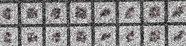
Fig. 10.1 A cryo-EM micrograph of beta-galactosidase particles in vitrified ice. Individual particles (bright and dark blobs) are visible, but a single micrograph contains too little SNR to resolve molecular detail. Combining images of many such particles through SPA reveals the protein structure at near-atomic resolution.

In the below video, we explain how a three-dimensional structure is recovered from many noisy projection images: back projection in real space, the equivalent route in Fourier space via the projection theorem, and the iterative single-particle workflow that leads from micrographs to a final Coulomb potential map.

---

---

10.2. Why Averaging Works: Signal and Noise

Individual cryo-EM particle images are collected at very low electron dose (typically 40–70 e⁻/Ų total per micrograph) to avoid radiation damage. As a consequence, each particle image is dominated by noise. The signal-to-noise ratio (SNR) of a single particle image is often less than 0.1 — the particle is literally invisible by eye in the raw image.

Averaging \(N\) images of identical particles, each containing the same underlying signal but independent noise, amplifies the signal by \(N\) while the noise grows only by \(\sqrt{N}\). The SNR therefore scales as:

(10.1)\[ \text{SNR}(N) = \text{SNR}(1) \times \sqrt{N} \]

This \(\sqrt{N}\) improvement is the statistical foundation of SPA. To improve SNR by a factor of 10, one needs 100 particles; a factor of 100 requires 10,000. Modern SPA datasets typically contain \(10^5\)–\(10^6\) particle images, yielding SNR improvements of 300–1000× over a single particle.

Interactive element

Click Live Code to activate, expand the Show code toggle, and click ▶ to run. Drag the slider to increase the number of averaged particles and observe how the ring feature becomes progressively clearer. Note that the SNR improvement follows \(\sqrt{N}\).

Show code cell source

Hide code cell source

import io
import numpy as np
import matplotlib
matplotlib.use('agg')
import matplotlib.pyplot as plt
from ipywidgets import IntSlider, FloatSlider, VBox, HBox, Layout, Output
from IPython.display import display, Image, clear_output

def draw_averaging(n_particles=16, noise_level=3.0):
    rng = np.random.default_rng(42)
    n = 80
    x = np.linspace(-1, 1, n)
    X, Y = np.meshgrid(x, x)
    r = np.sqrt(X**2 + Y**2)
    particle = np.exp(-((r - 0.55)**2)/(2*0.06**2)) + 0.3*np.exp(-(r**2)/(2*0.10**2))
    particle /= particle.max()

    imgs = particle[None] + rng.normal(0, noise_level, (n_particles, n, n))
    avg  = imgs.mean(axis=0)
    vscale = noise_level * 1.5

    fig, axes = plt.subplots(1, 4, figsize=(12, 3.2))
    axes[0].imshow(particle, cmap='gray', vmin=0, vmax=1)
    axes[0].set_title("True structure", fontsize=10); axes[0].axis('off')
    axes[1].imshow(imgs[0], cmap='gray', vmin=-vscale, vmax=vscale)
    axes[1].set_title("Single particle image", fontsize=10); axes[1].axis('off')
    axes[2].imshow(imgs[:min(4,n_particles)].mean(0), cmap='gray', vmin=-vscale, vmax=vscale)
    axes[2].set_title(f"Average of {min(4,n_particles)}", fontsize=10); axes[2].axis('off')
    axes[3].imshow(avg, cmap='gray', vmin=-vscale, vmax=vscale)
    axes[3].set_title(f"Average of {n_particles}\n(SNR ∝ {np.sqrt(n_particles):.1f}×)", fontsize=10)
    axes[3].axis('off')
    fig.tight_layout()
    buf = io.BytesIO(); fig.savefig(buf, format='png', dpi=96); buf.seek(0)
    display(Image(data=buf.read())); plt.close(fig)

style = {"description_width": "150px"}
sl = Layout(width="360px")
n_sl    = IntSlider(  value=16,  min=1,   max=512, step=1,
                       description="# particles", style=style, layout=sl)
nse_sl  = FloatSlider(value=3.0, min=0.5, max=8.0, step=0.5,
                       description="Noise level",  style=style, layout=sl)

out = Output()
def update_avg(_=None):
    with out:
        clear_output(wait=True)
        draw_averaging(n_sl.value, nse_sl.value)
for sl_w in [n_sl, nse_sl]:
    sl_w.observe(update_avg, names='value')

ui = VBox([n_sl, nse_sl])
display(HBox([ui, out]))
update_avg()

10.3. The 2D Reconstruction Problem

Before explaining the full SPA pipeline, it is instructive to work through the problem in 2D, where the unknown structure is a 2D image and the only unknown parameter per particle is a single in-plane rotation angle. This makes the algorithm concrete and computable in a browser. The same logic applies in 3D — the only difference is that we search over three Euler angles instead of one.

10.3.1. The Observation Model

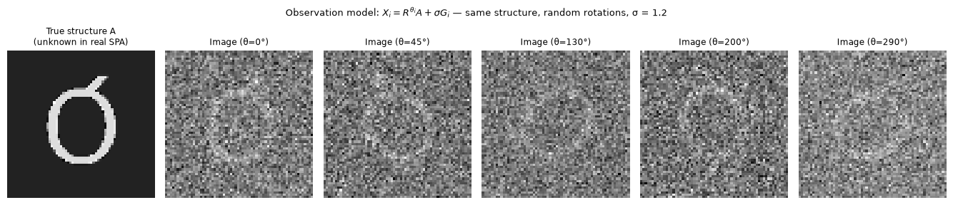
We model each observed particle image \(X_i\) as a rotated, noise-corrupted version of an unknown density \(A\):

(10.2)\[ X_i = R^{\theta_i} A + \sigma G_i \]

where \(R^{\theta_i}\) denotes rotation by the unknown angle \(\theta_i\), and \(G_i\) is i.i.d. Gaussian noise with standard deviation \(\sigma\). Neither \(A\) nor any of the \(\theta_i\) are known. If we could estimate \(\theta_i\), we could recover \(A\) by rotating each image back and averaging:

(10.3)\[ A \approx \frac{1}{N} \sum_{i=1}^N (R^{\theta_i})^{-1} X_i \]

This partially cancels the noise (by \(\sqrt{N}\)) while the signal adds coherently — provided the angle estimates are correct.

We use a rendition of the letter Q as our 2D particle throughout, because it has clear asymmetry (making correct alignment unambiguous) and is immediately recognisable in the reconstruction. In real SPA the structure is of course unknown.

10.3.2. Alignment by Cross-Correlation

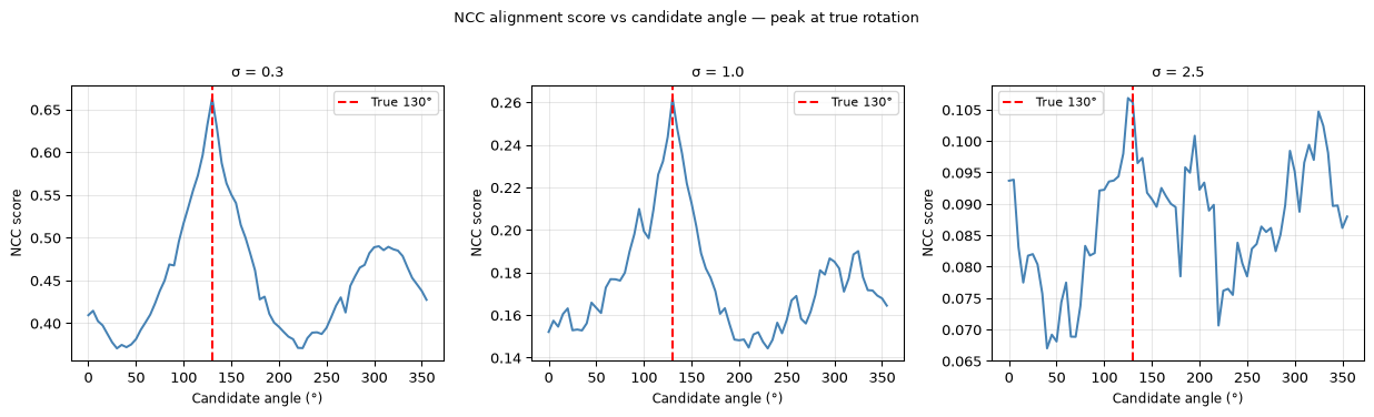
To estimate \(\theta_i\) we compare each image against a reference (an estimate of \(A\)) rotated to all candidate angles. The normalised cross-correlation (NCC) between image \(X_i\) and a candidate rotated reference \(R^\theta A_\text{ref}\) is:

\[ \mathrm{NCC}(\theta) = \frac{\sum_\mathbf{r} X_i(\mathbf{r})\, [R^\theta A_\text{ref}](\mathbf{r})} {\|X_i\|\,\|R^\theta A_\text{ref}\|} \]

The estimated angle is \(\hat\theta_i = \arg\max_\theta \mathrm{NCC}(\theta)\). The figure below shows the NCC score as a function of candidate angle for a single noisy image. Even at substantial noise levels, a clear peak is visible near the true angle.

10.3.3. Live 2D Reconstruction

The interactive below runs the complete pipeline. At startup, 36 rotated references are pre-computed at 10° steps. Each slider update:

1. Generates N noisy rotated images of Q

2. Aligns each image against all 36 references (vectorised NCC)

3. Rotates each image back by its estimated angle

4. Averages all aligned images

Interactive element

Click Live Code to activate, expand the Show code toggle, and click ▶ to run. Increase particle images to watch Q emerge from noise. Raise noise to see alignment fail when the NCC peak is too broad.

Show code cell source

Hide code cell source

import io
import numpy as np
import matplotlib
matplotlib.use('agg')
import matplotlib.pyplot as plt
from scipy.ndimage import rotate as nd_rotate, zoom as nd_zoom
from ipywidgets import IntSlider, FloatSlider, VBox, Output
from IPython.display import display, Image, clear_output

def make_letter(text, size=64):
    fig, ax = plt.subplots(figsize=(2, 2))
    ax.axis('off')
    fig.text(0.23, 0.26, text, fontsize=100)
    fig.canvas.draw()
    buf = np.frombuffer(fig.canvas.buffer_rgba(), dtype=np.uint8)
    w, h = fig.canvas.get_width_height()
    data = buf.reshape(h, w, 4)[:, :, :3].mean(2)
    plt.close(fig)
    data = (data - data.min()) / (data.max() - data.min() + 1e-10)
    data = (~data.astype(bool))[::-1].astype(float)
    return nd_zoom(data, size / data.shape[0])

_pm_ref  = make_letter('Q', 64)
_pm_n    = 64
_pm_cand = np.arange(0, 360, 10)
_pm_rots = np.array([nd_rotate(_pm_ref, a, reshape=False, order=1) for a in _pm_cand])

def _ncc_mat(imgs, refs):
    ni, px = imgs.shape[0], imgs.shape[1]*imgs.shape[2]
    A = imgs.reshape(ni, px).astype(float); A -= A.mean(1, keepdims=True)
    B = refs.reshape(len(refs), px).astype(float); B -= B.mean(1, keepdims=True)
    An = np.linalg.norm(A, axis=1, keepdims=True).clip(1e-10)
    Bn = np.linalg.norm(B, axis=1, keepdims=True).clip(1e-10)
    with np.errstate(divide='ignore', invalid='ignore', over='ignore'):
        return np.nan_to_num((A/An) @ (B/Bn).T)

def draw_pm_recon(n_images=32, noise_sigma=1.0):
    rng = np.random.default_rng(7)
    idx   = rng.integers(0, len(_pm_cand), n_images)
    noisy = _pm_rots[idx] + rng.normal(0, noise_sigma, (n_images, _pm_n, _pm_n))
    best  = _ncc_mat(noisy, _pm_rots).argmax(1)

    recon = np.zeros((_pm_n, _pm_n))
    for a_idx in range(len(_pm_cand)):
        mask = (best == a_idx)
        if mask.any():
            recon += nd_rotate(noisy[mask].mean(0), -_pm_cand[a_idx],
                               reshape=False, order=1) * mask.sum()
    recon /= n_images

    r_n = (recon - recon.mean()) / (recon.std() + 1e-10)
    t_n = (_pm_ref - _pm_ref.mean()) / (_pm_ref.std() + 1e-10)
    ncc_val = float((r_n * t_n).mean())

    # NCC scores for first image
    px = _pm_n * _pm_n
    A0 = noisy[0].reshape(1, px).astype(float); A0 -= A0.mean()
    A0n = np.linalg.norm(A0).clip(1e-10)
    B0 = _pm_rots.reshape(len(_pm_cand), px).astype(float); B0 -= B0.mean(1, keepdims=True)
    B0n = np.linalg.norm(B0, axis=1, keepdims=True).clip(1e-10)
    with np.errstate(divide='ignore', invalid='ignore', over='ignore'):
        scores0 = np.nan_to_num(((A0/A0n) @ (B0/B0n).T).ravel())

    fig, axes = plt.subplots(1, 5, figsize=(18, 3.8))
    axes[0].imshow(_pm_ref, cmap='gray'); axes[0].axis('off')
    axes[0].set_title("True structure\n(unknown in real SPA)", fontsize=9)

    vr = noise_sigma * 1.5
    axes[1].imshow(noisy[0], cmap='gray', vmin=-vr, vmax=vr); axes[1].axis('off')
    axes[1].set_title(f"Single image (σ={noise_sigma:.1f})", fontsize=9)

    axes[2].plot(_pm_cand, scores0, color='steelblue', linewidth=1.4)
    axes[2].axvline(_pm_cand[best[0]], color='red', linewidth=1.4, linestyle='--',
                    label=f'Best: {_pm_cand[best[0]]}°')
    axes[2].set_xlabel("Candidate angle (°)", fontsize=8)
    axes[2].set_ylabel("NCC", fontsize=8)
    axes[2].set_title("Alignment score\n(image 1)", fontsize=9)
    axes[2].legend(fontsize=7); axes[2].grid(alpha=0.3)

    aligned0 = nd_rotate(noisy[0], -_pm_cand[best[0]], reshape=False, order=1)
    axes[3].imshow(aligned0, cmap='gray', vmin=-vr, vmax=vr); axes[3].axis('off')
    axes[3].set_title(f"Image 1 aligned\n(rotated back {_pm_cand[best[0]]}°)", fontsize=9)

    vr2 = max(abs(recon).max(), 0.01)
    axes[4].imshow(recon, cmap='gray', vmin=-vr2, vmax=vr2); axes[4].axis('off')
    axes[4].set_title(f"Reconstruction ({n_images} images)\nNCC quality: {ncc_val:.2f}", fontsize=9)

    fig.suptitle("2D projection-matching reconstruction", fontsize=10)
    fig.tight_layout()
    buf = io.BytesIO(); fig.savefig(buf, format='png', dpi=96); buf.seek(0)
    display(Image(data=buf.read())); plt.close(fig)

style = {"description_width": "160px"}
n_sl_pm   = IntSlider(value=32, min=4, max=128, step=4,
                      description="# particle images", style=style, layout={"width":"440px"})
nse_sl_pm = FloatSlider(value=1.0, min=0.2, max=4.0, step=0.2,
                        description="Noise σ", style=style, layout={"width":"440px"})

out_pm = Output()
def update_pm(_=None):
    with out_pm:
        clear_output(wait=True)
        draw_pm_recon(n_sl_pm.value, nse_sl_pm.value)
for s in [n_sl_pm, nse_sl_pm]:
    s.observe(update_pm, names='value')

display(VBox([n_sl_pm, nse_sl_pm, out_pm]))
update_pm()

10.4. Model Bias and Reference Dependence

The projection-matching algorithm requires a starting reference to align images against. In real SPA this reference is often a low-resolution density map from a previous processing round, an electron microscopy structure of a homologous protein, or a featureless sphere. The choice of starting reference matters: if the reference is wrong, the alignment may converge to the wrong structure — a phenomenon called reference bias or the “Einstein from noise” problem.

The example below illustrates three cases for reconstructing images of the letter Q:

• Correct reference (Q): alignment converges immediately; reconstruction is faithful.

• Wrong reference (P): particles are forced into P-like alignments; the reconstruction is a blend of Q and P.

• Neutral reference (circle): no bias is introduced, but convergence is slower because the reference provides less discriminating power.

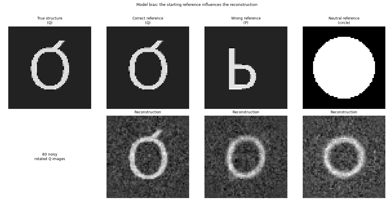
This demonstration has an important practical implication: in real SPA, reconstructions should always be validated by checking that two independently processed half-datasets give the same structure (the gold-standard FSC criterion). A structure that matches its own reference but not an independent test set may be a result of reference bias rather than a genuine structural signal.

The remedy is iterative refinement: use the reconstruction from one round as the reference for the next. Starting from a neutral reference and iterating, the algorithm gradually converges to the correct structure without being biased toward a specific starting model.

10.5. 2D Classification

Real cryo-EM datasets are not homogeneous: micrographs contain ice contamination, broken particles, aggregates, and sometimes multiple distinct conformations of the protein. 2D classification solves two problems simultaneously:

1. Quality control: junk particles form diffuse, uninterpretable classes and can be discarded.

2. Sorting by view: particles in the same orientation are grouped together, producing high-SNR class averages.

The algorithm is analogous to the single-class reconstruction above, but extended to \(K\) classes. For each particle, we compute NCC against all rotations of all \(K\) references, and assign the particle to the best-matching class and angle. References are then updated as averages of their assigned particles.

The example below mixes images of two different letters — Q and P — and shows that the algorithm correctly separates them into two distinct classes, even though we are working blindly (the algorithm receives no information about which images belong to which class).

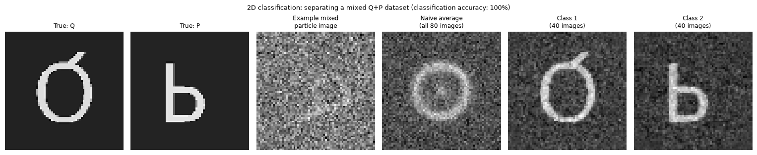
The interactive below lets you explore how noise and number of images affect classification. At low noise the two letters are cleanly separated; at high noise, assignments become unreliable and the class averages deteriorate.

Interactive element

Click Live Code to activate, expand the Show code toggle, and click ▶ to run. Adjust the noise level and the number of images per class and observe how class separation changes.

Show code cell source

Hide code cell source

import io
import numpy as np
import matplotlib
matplotlib.use('agg')
import matplotlib.pyplot as plt
from scipy.ndimage import rotate as nd_rotate, zoom as nd_zoom
from ipywidgets import IntSlider, FloatSlider, VBox, Output
from IPython.display import display, Image, clear_output

def make_letter(text, size=64):
    fig, ax = plt.subplots(figsize=(2, 2))
    ax.axis('off')
    fig.text(0.23, 0.26, text, fontsize=100)
    fig.canvas.draw()
    buf = np.frombuffer(fig.canvas.buffer_rgba(), dtype=np.uint8)
    w, h = fig.canvas.get_width_height()
    data = buf.reshape(h, w, 4)[:, :, :3].mean(2)
    plt.close(fig)
    data = (data - data.min()) / (data.max() - data.min() + 1e-10)
    data = (~data.astype(bool))[::-1].astype(float)
    return nd_zoom(data, size / data.shape[0])

_cls_Q = make_letter('Q', 64)
_cls_P = make_letter('P', 64)
_cls_cand = np.arange(0, 360, 10)
_rots_Q = np.array([nd_rotate(_cls_Q, a, reshape=False, order=1) for a in _cls_cand])
_rots_P = np.array([nd_rotate(_cls_P, a, reshape=False, order=1) for a in _cls_cand])
_all_rots = np.concatenate([_rots_Q, _rots_P])
_n_cand = len(_cls_cand)
_px = 64*64

def draw_classification(n_each=40, sigma=1.2):
    rng = np.random.default_rng(42)
    idx_q = rng.integers(0, _n_cand, n_each)
    idx_p = rng.integers(0, _n_cand, n_each)
    imgs_q = _rots_Q[idx_q] + rng.normal(0, sigma, (n_each, 64, 64))
    imgs_p = _rots_P[idx_p] + rng.normal(0, sigma, (n_each, 64, 64))
    all_imgs = np.concatenate([imgs_q, imgs_p])
    true_lbl = np.array([0]*n_each + [1]*n_each)
    shuf = rng.permutation(2*n_each)
    all_imgs = all_imgs[shuf]; true_lbl = true_lbl[shuf]

    n_all = all_imgs.shape[0]
    A = all_imgs.reshape(n_all, _px).astype(float); A -= A.mean(1, keepdims=True)
    B = _all_rots.reshape(len(_all_rots), _px).astype(float); B -= B.mean(1, keepdims=True)
    An = np.linalg.norm(A, axis=1, keepdims=True).clip(1e-10)
    Bn = np.linalg.norm(B, axis=1, keepdims=True).clip(1e-10)
    with np.errstate(divide='ignore', invalid='ignore', over='ignore'):
        cc = np.nan_to_num((A/An) @ (B/Bn).T)
    best_global = cc.argmax(1)
    pred_cls  = (best_global >= _n_cand).astype(int)
    best_ang  = _cls_cand[best_global % _n_cand]
    acc = (pred_cls == true_lbl).mean() * 100

    recons = []
    for ci in [0, 1]:
        mask = (pred_cls == ci)
        recon = np.zeros((64, 64))
        count = 0
        for i in np.where(mask)[0]:
            recon += nd_rotate(all_imgs[i], -best_ang[i], reshape=False, order=1)
            count += 1
        recons.append(recon / max(count, 1))

    naive = all_imgs.mean(0)
    fig, axes = plt.subplots(1, 5, figsize=(16, 3.6))
    axes[0].imshow(all_imgs[0], cmap='gray'); axes[0].axis('off')
    axes[0].set_title(f"Example image\n(σ={sigma:.1f}, N={2*n_each} total)", fontsize=9)
    axes[1].imshow(naive, cmap='gray'); axes[1].axis('off')
    axes[1].set_title("Naive average\n(mixed → blurry)", fontsize=9)
    axes[2].imshow(recons[0], cmap='gray'); axes[2].axis('off')
    axes[2].set_title(f"Class 1 ({(pred_cls==0).sum()} imgs)", fontsize=9)
    axes[3].imshow(recons[1], cmap='gray'); axes[3].axis('off')
    axes[3].set_title(f"Class 2 ({(pred_cls==1).sum()} imgs)", fontsize=9)
    axes[4].imshow(np.abs(recons[0] - recons[1]), cmap='hot'); axes[4].axis('off')
    axes[4].set_title("Difference\n(class 1 − class 2)", fontsize=9)
    fig.suptitle(f"2D classification accuracy: {acc:.0f}%", fontsize=10)
    fig.tight_layout()
    buf = io.BytesIO(); fig.savefig(buf, format='png', dpi=96); buf.seek(0)
    display(Image(data=buf.read())); plt.close(fig)

style = {"description_width": "160px"}
n_sl_cls  = IntSlider(value=40, min=8, max=100, step=4,
                      description="Images per class", style=style, layout={"width":"440px"})
sig_sl_cls = FloatSlider(value=1.2, min=0.2, max=4.0, step=0.2,
                         description="Noise σ", style=style, layout={"width":"440px"})
out_cls = Output()
def update_cls(_=None):
    with out_cls:
        clear_output(wait=True)
        draw_classification(n_sl_cls.value, sig_sl_cls.value)
for s in [n_sl_cls, sig_sl_cls]:
    s.observe(update_cls, names='value')
display(VBox([n_sl_cls, sig_sl_cls, out_cls]))
update_cls()

10.6. Maximum-Likelihood Alignment

At the SNR typical of cryo-EM images (0.01–0.1), the NCC peak is broad and noisy: many candidate orientations give nearly equal scores (see Section 8.5). Hard assignment of the single best-fit orientation ignores this uncertainty and introduces systematic bias.

Maximum-likelihood (ML) alignment resolves this by treating orientations as a probability distribution. Given the observation model in (10.2), and assuming Gaussian noise with variance \(\sigma^2\), the probability of observing \(X_i\) given orientation \(\theta_j\) and reference \(A\) is:

\[ P(X_i \mid \theta_j, A) \propto \exp\!\left[-\frac{\|X_i - R^{\theta_j} A\|^2}{2\sigma^2}\right] = \exp\!\left[\frac{\mathrm{CC}(\theta_j)}{\sigma^2}\right] \cdot \mathrm{const} \]

The posterior probability of each orientation is:

\[ w_{ij} = P(\theta_j \mid X_i, A) = \frac{P(X_i \mid \theta_j, A)}{\sum_{j'} P(X_i \mid \theta_{j'}, A)} \]

These weights \(w_{ij}\) are soft assignments: at high SNR they collapse onto the single best orientation (recovering projection matching), but at low SNR they spread over many orientations, giving each a contribution proportional to its likelihood. The reconstruction is then a weighted average:

\[ A \leftarrow \sum_i \sum_j w_{ij} \, (R^{\theta_j})^{-1} X_i \]

This is one step of the expectation-maximization (EM) algorithm: the E-step computes the weights \(w_{ij}\) from the current reference \(A\); the M-step reconstructs \(A\) from the weighted back-projections. Iterating E and M steps converges to the maximum-likelihood estimate of \(A\).

The key advantages of ML over hard projection matching are: (1) alignment uncertainty at low SNR is automatically accounted for; (2) the reconstruction is less susceptible to reference bias; and (3) conformational heterogeneity can be modelled by introducing multiple reference classes, with particles assigned soft weights to each class.

10.7. The SPA Workflow

10.7.1. Specimen Preparation

SPA requires a purified, monodisperse sample of the macromolecule of interest in an appropriate buffer. A 3–4 µL aliquot is applied to a TEM grid covered with a support film containing micrometer-scale holes. Excess liquid is blotted away and the grid is plunge-frozen in liquid ethane using a vitrification robot. Preferred ice thickness is typically 10–100 nm.

10.7.2. Automated Data Collection

Automated acquisition software handles focusing, image shift, and stage movement to collect thousands of micrographs. A typical session collects 1,000–10,000 micrographs per day, each containing tens to hundreds of individual particle images. Data collection follows a strict low-dose protocol: total dose is 40–70 e⁻/Ų per micrograph, spread over 30–60 movie frames.

10.7.3. Preprocessing

Motion correction: frames of each movie are aligned and averaged using cross-correlation to correct beam-induced motion.

CTF estimation: defocus and astigmatism are estimated from each micrograph’s power spectrum for later correction.

Particle picking: individual particle images are identified using neural-network-based pickers that find particles in noisy images without user-defined templates.

10.7.4. Fourier Reconstruction

Once orientations are assigned, the 3D reconstruction is computed via Fourier inversion. By the projection slice theorem (discussed in Section 9), the 2D Fourier transform of each projection is a central slice through the 3D Fourier transform of the object. Inserting all 2D Fourier transforms as oriented slices into a 3D Fourier volume, and then inverse-Fourier-transforming, yields the 3D density map. SPA benefits from the near-complete angular coverage provided by particles in random orientations — unlike tomography, there is no systematic missing wedge.

10.7.5. Conformational Heterogeneity

3D classification can sort particles into discrete conformational states, each yielding a separate map. Continuous flexibility is handled by methods such as 3D variability analysis or multi-body refinement.

10.8. Resolution Assessment: The Fourier Shell Correlation

10.8.1. FSC Definition

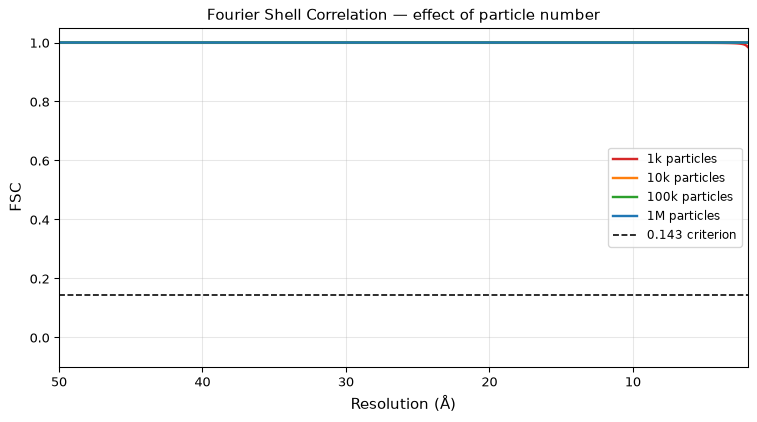
The resolution of a cryo-EM map is assessed using the Fourier Shell Correlation (FSC). The dataset is split randomly into two equal halves, and two independent 3D maps are computed from each half. The FSC between the two half-maps as a function of spatial frequency \(s\) is:

(10.4)\[ \text{FSC}(s) = \frac{\sum_{\mathbf{k} \in \text{shell}(s)} F_1(\mathbf{k})\, F_2^*(\mathbf{k})}{\sqrt{\sum |F_1|^2 \sum |F_2|^2}} \]

The FSC is 1 at low frequencies (both half-maps agree) and falls toward 0 at high frequencies (pure noise). The gold-standard resolution is defined as the frequency at which the FSC crosses 0.143 — a criterion chosen so that the map SNR equals approximately 1 at that frequency.

10.9. Biological Applications

SPA has transformed structural biology:

• Ribosomes (2.0–2.5 Å): the bacterial ribosome provided an early proof-of-concept for high-resolution SPA and remains a benchmark dataset.

• Ion channels and membrane proteins: the TRPV1 channel was among the first membrane proteins solved to near-atomic resolution by cryo-EM.

• Viruses: large icosahedral viruses leverage high symmetry for near-atomic resolution with relatively few particles.

• Drug targets: rapid structure determination of viral spike proteins and other therapeutic targets.

The method continues to push toward harder targets: smaller proteins (\(< 50\) kDa), flexible complexes, and specimens in their native cellular environment (in-situ cryo-ET, see Section 11).