9. Fourier Analysis in Imaging

The Fourier transform is the single most important mathematical tool in quantitative imaging. It provides a language for describing images in terms of their spatial frequency content — which periodicities are present, at what amplitude, and at what phase. Understanding Fourier analysis is essential for making sense of resolution, contrast, filtering, and the tomographic reconstruction methods described in Section 11.

9.1. The 1D Fourier Transform

Any periodic signal can be decomposed into a sum of sinusoids — this is the central insight of Fourier analysis. For a non-periodic signal, the continuous Fourier transform generalises this to a continuous integral:

(9.1)\[ \hat{f}(\nu) = \int_{-\infty}^{\infty} f(x)\, e^{-2\pi i \nu x}\, dx \]

where \(f(x)\) is the signal in real space (e.g., position \(x\)), \(\hat{f}(\nu)\) is its Fourier transform in frequency space, and \(\nu\) is the spatial frequency (cycles per unit length). The inverse transform recovers the original signal:

(9.2)\[ f(x) = \int_{-\infty}^{\infty} \hat{f}(\nu)\, e^{2\pi i \nu x}\, d\nu \]

The Fourier transform \(\hat{f}(\nu)\) is in general complex. Its magnitude \(|\hat{f}(\nu)|\) is the amplitude spectrum, and \(\arg \hat{f}(\nu)\) is the phase spectrum. The power spectrum is \(|\hat{f}(\nu)|^2\).

9.1.1. Key Properties

Property	Real space	Fourier space
Linearity	\(a f + b g\)	\(a\hat{f} + b\hat{g}\)
Shift	\(f(x - x_0)\)	\(e^{-2\pi i \nu x_0}\hat{f}(\nu)\) — phase shift only
Scale	\(f(ax)\)	\(\frac{1}{|a|}\hat{f}(\nu/a)\) — wide → narrow, narrow → wide
Convolution	\(f * g\)	\(\hat{f} \cdot \hat{g}\) — convolution becomes multiplication
Parseval	\(\int |f|^2 dx\)	\(\int |\hat{f}|^2 d\nu\) — energy is conserved

The convolution theorem is particularly important for imaging: the action of any linear, shift-invariant imaging system (a lens, a detector, a filter) can be described by its point spread function (PSF) in real space, or equivalently by its transfer function (the Fourier transform of the PSF) in frequency space. Multiplying in frequency space is far more efficient than convolving in real space for large images.

The interactive below lets you build a 1D signal from sinusoidal components and see the resulting power spectrum. Adding components of different frequencies, amplitudes, and phases shows how complex waveforms arise from simple harmonic building blocks.

Interactive element

Click Live Code to activate, expand the Show code toggle, and click ▶ to run. Use the sliders to adjust the frequencies and amplitudes of three sine-wave components. The signal panel shows the resulting waveform; the spectrum panel shows its power spectrum.

Show code cell source

Hide code cell source

import io
import numpy as np
import matplotlib
matplotlib.use('agg')
import matplotlib.pyplot as plt
from ipywidgets import FloatSlider, IntSlider, VBox, HBox, Output, Label
from IPython.display import display, Image, clear_output

_x = np.linspace(0, 1, 512)
_freqs = np.fft.rfftfreq(512, d=1/512)

def draw_1d_ft(f1=1, A1=1.0, f2=3, A2=0.5, f3=7, A3=0.25):
    sig = (A1 * np.sin(2*np.pi*f1*_x) +
           A2 * np.sin(2*np.pi*f2*_x) +
           A3 * np.sin(2*np.pi*f3*_x))
    ps = np.abs(np.fft.rfft(sig))**2 / 512

    fig, (ax1, ax2) = plt.subplots(1, 2, figsize=(13, 4))
    ax1.plot(_x, sig, color='steelblue', linewidth=2)
    ax1.set_xlabel("Position x", fontsize=10)
    ax1.set_ylabel("Signal amplitude", fontsize=10)
    ax1.set_title("Signal (sum of three sinusoids)", fontsize=10)
    ax1.grid(alpha=0.3)

    ax2.stem(_freqs[:30], ps[:30], linefmt='C1-', markerfmt='C1o', basefmt='k-')
    ax2.set_xlabel("Spatial frequency (cycles)", fontsize=10)
    ax2.set_ylabel("Power", fontsize=10)
    ax2.set_title("Power spectrum", fontsize=10)
    ax2.grid(alpha=0.3)

    fig.tight_layout()
    buf = io.BytesIO(); fig.savefig(buf, format='png', dpi=96); buf.seek(0)
    display(Image(data=buf.read())); plt.close(fig)

style = {"description_width": "80px"}
sl_kw = {"layout": {"width": "320px"}}
f1_sl = IntSlider(value=1,  min=1, max=15, step=1,  description="Freq 1", style=style, **sl_kw)
A1_sl = FloatSlider(value=1.0, min=0.0, max=2.0, step=0.1, description="Amp 1",  style=style, **sl_kw)
f2_sl = IntSlider(value=3,  min=1, max=20, step=1,  description="Freq 2", style=style, **sl_kw)
A2_sl = FloatSlider(value=0.5, min=0.0, max=2.0, step=0.1, description="Amp 2",  style=style, **sl_kw)
f3_sl = IntSlider(value=7,  min=1, max=25, step=1,  description="Freq 3", style=style, **sl_kw)
A3_sl = FloatSlider(value=0.25, min=0.0, max=2.0, step=0.1, description="Amp 3", style=style, **sl_kw)

out_1d = Output()
def update_1d(_=None):
    with out_1d:
        clear_output(wait=True)
        draw_1d_ft(f1_sl.value, A1_sl.value, f2_sl.value, A2_sl.value, f3_sl.value, A3_sl.value)
for s in [f1_sl, A1_sl, f2_sl, A2_sl, f3_sl, A3_sl]:
    s.observe(update_1d, names='value')

display(VBox([HBox([VBox([f1_sl, A1_sl]), VBox([f2_sl, A2_sl]), VBox([f3_sl, A3_sl])]), out_1d]))
update_1d()

9.2. The 2D Fourier Transform in Images

For a 2D image \(f(x, y)\), the Fourier transform extends naturally to two dimensions:

(9.3)\[ \hat{f}(k_x, k_y) = \iint f(x, y)\, e^{-2\pi i (k_x x + k_y y)}\, dx\, dy \]

Here \((k_x, k_y)\) are the two components of the spatial frequency vector \(\mathbf{k}\). The magnitude \(|\mathbf{k}| = \sqrt{k_x^2 + k_y^2}\) is the radial spatial frequency (1/resolution), and the direction of \(\mathbf{k}\) indicates the orientation of the corresponding sinusoidal pattern in the image.

9.2.1. Interpreting the 2D FT

After applying fftshift to move the DC component (zero frequency) to the centre, the 2D FT has a characteristic structure:

• Centre (DC component): the average value of the image

• Near centre (low frequencies): coarse structure, global intensity variation

• Away from centre (high frequencies): fine detail, sharp edges

• Bright lines or arcs: features with a strong periodic structure at that frequency and orientation

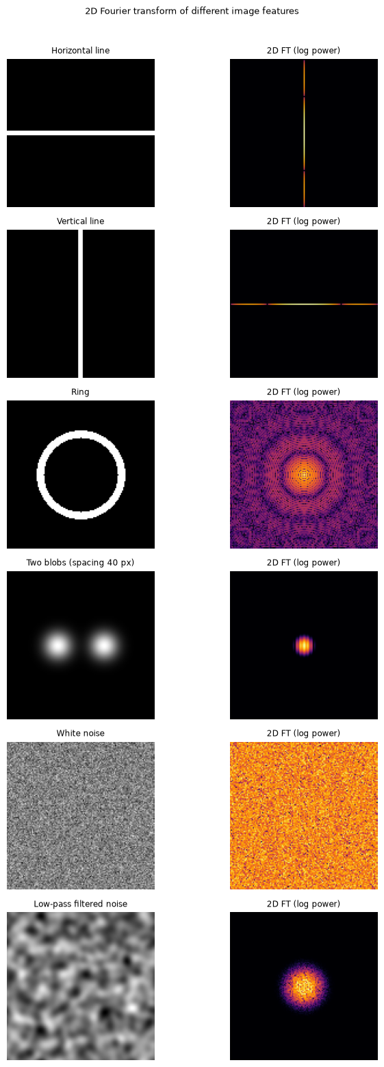
Several important image features have recognisable signatures in the 2D FT:

• A horizontal line in the image appears as a vertical line in the FT (perpendicular to the feature)

• A dot (isotropic blob) appears as a ring in the FT

• A ring in the image appears as a ring in the FT (at the reciprocal radius)

9.3. Filtering in Fourier Space

Because convolution in real space equals multiplication in Fourier space (the convolution theorem), spatial filtering — suppressing or enhancing certain frequencies — is most easily implemented by multiplying the 2D FT by a filter function \(H(k_x, k_y)\) and then inverse-transforming:

(9.4)\[ g(x, y) = \mathcal{F}^{-1}\!\left[ H(k_x, k_y) \cdot \hat{f}(k_x, k_y) \right] \]

Common filter types:

Low-pass filter: \(H = 1\) for \(|\mathbf{k}| < k_\text{cut}\), \(H = 0\) otherwise. Attenuates high frequencies → smooths the image, removes noise but also blurs detail. In cryo-EM, low-pass filtering is used to remove high-frequency noise from noisy micrographs.

High-pass filter: \(H = 0\) for \(|\mathbf{k}| < k_\text{cut}\), \(H = 1\) otherwise. Attenuates low frequencies → enhances edges and fine detail, but amplifies high-frequency noise. The ramp filter used in filtered backprojection (see Section 11) is a radial high-pass filter \(H = |\mathbf{k}|\).

Band-pass filter: passes a range of frequencies. Used for specific feature enhancement (e.g., suppressing both very low and very high frequencies while retaining intermediate-scale structures).

A sharp cutoff in Fourier space (a “top-hat” filter) causes ringing artifacts (Gibbs phenomenon) in real space. In practice, filters are smoothed with a Gaussian or cosine taper. The choice of filter shape involves a trade-off between frequency selectivity and real-space artifacts.

Interactive element

Click Live Code to activate, expand the Show code toggle, and click ▶ to run. Choose a filter type and adjust the cutoff frequency. Watch how the image changes and what the Fourier-space filter looks like.

Show code cell source

Hide code cell source

import io
import numpy as np
import matplotlib
matplotlib.use('agg')
import matplotlib.pyplot as plt
from ipywidgets import FloatSlider, Dropdown, VBox, HBox, Output
from IPython.display import display, Image, clear_output

def _make_ti(n=128):
    y, x = np.mgrid[0:n, 0:n].astype(float)
    cx, cy = n/2, n/2
    img = np.zeros((n, n))
    R = np.sqrt((x-cx)**2 + (y-cy)**2)
    img += 0.8 * ((R > 0.22*n) & (R < 0.28*n)).astype(float)
    img += 0.9 * (np.abs(y - cy*1.5) < n*0.02).astype(float)
    img += 0.7 * (np.sqrt((x-cx*1.6)**2+(y-cy*0.5)**2) < n*0.06).astype(float)
    img += 0.05 * np.random.default_rng(1).standard_normal((n, n))
    return np.clip(img, 0, 1)

_fil_img = _make_ti(128)
_fil_n = 128
kx = np.fft.fftfreq(_fil_n); ky = np.fft.fftfreq(_fil_n)
_KX, _KY = np.meshgrid(kx, ky); _K = np.sqrt(_KX**2 + _KY**2)
_FT = np.fft.fft2(_fil_img)

def draw_filter(filter_type='Low-pass', cutoff=0.15):
    if filter_type == 'Low-pass':
        H = np.exp(-(_K/cutoff)**4)
        label = f"Low-pass (cutoff={cutoff:.2f})"
    elif filter_type == 'High-pass':
        H = 1 - np.exp(-(_K/cutoff)**4)
        label = f"High-pass (cutoff={cutoff:.2f})"
    else:
        H = _K / _K.max()
        label = "Ramp filter |k|"

    filtered = np.real(np.fft.ifft2(_FT * np.fft.ifftshift(H)))
    H_display = np.fft.fftshift(H)

    fig, axes = plt.subplots(1, 4, figsize=(16, 4.2))
    axes[0].imshow(_fil_img, cmap='gray'); axes[0].axis('off')
    axes[0].set_title("Original image", fontsize=9)
    axes[1].imshow(np.log1p(np.abs(np.fft.fftshift(_FT))), cmap='inferno'); axes[1].axis('off')
    axes[1].set_title("2D FT (log power)", fontsize=9)
    axes[2].imshow(H_display, cmap='RdBu_r', vmin=0, vmax=1); axes[2].axis('off')
    axes[2].set_title(f"Filter H(k)\n{label}", fontsize=9)
    axes[3].imshow(filtered, cmap='gray'); axes[3].axis('off')
    axes[3].set_title("Filtered image", fontsize=9)

    fig.suptitle(f"Fourier filtering: {label}", fontsize=10)
    fig.tight_layout()
    buf = io.BytesIO(); fig.savefig(buf, format='png', dpi=96); buf.seek(0)
    display(Image(data=buf.read())); plt.close(fig)

filter_dd = Dropdown(options=['Low-pass', 'High-pass', 'Ramp'],
                     value='Low-pass', description='Filter type:',
                     style={"description_width": "110px"}, layout={"width": "280px"})
cutoff_sl = FloatSlider(value=0.15, min=0.02, max=0.48, step=0.01,
                        description="Cutoff k",
                        style={"description_width": "90px"}, layout={"width": "340px"})
out_fil = Output()
def update_fil(_=None):
    with out_fil:
        clear_output(wait=True)
        draw_filter(filter_dd.value, cutoff_sl.value)
for w in [filter_dd, cutoff_sl]:
    w.observe(update_fil, names='value')
display(VBox([HBox([filter_dd, cutoff_sl]), out_fil]))
update_fil()

9.4. Resolution and the Frequency Limit

In any digital image, the maximum representable spatial frequency is set by the pixel size (the Nyquist limit): if the pixel size is \(d\) (in Å/pixel), the highest frequency is \(\nu_\text{max} = 1/(2d)\) Å⁻¹. This is the Nyquist frequency. Features finer than \(2d\) cannot be represented in the image — they alias back to lower frequencies.

In cryo-EM, the nominal resolution is often defined as the spatial frequency at which the signal-to-noise ratio drops to 1, typically measured by the Fourier Shell Correlation (see Section 10.8.1). A map at “3 Å resolution” means the FSC drops below the 0.143 criterion at \(1/3\) Å⁻¹.

9.5. The Point Spread Function and the CTF

Every real imaging system has a point spread function (PSF): the image of a perfect point source. By the convolution theorem, the image of any object \(f\) through a system with PSF \(h\) is:

\[ g = f * h \quad \Longleftrightarrow \quad \hat{g} = \hat{f} \cdot \hat{h} \]

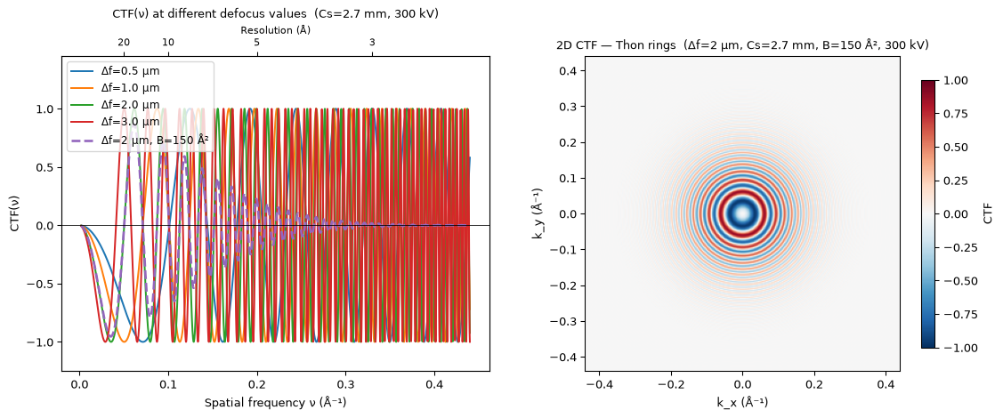
The Fourier transform of the PSF is the optical transfer function (OTF). For an electron microscope operating in phase-contrast mode, the OTF reduces to the contrast transfer function (CTF). The full derivation — starting from the weak phase object approximation and the wave-propagation picture of defocus-induced contrast — is given in Section 7.4. The result is:

\[ \mathrm{CTF}(\nu) = -\sin\!\left[\pi\lambda\Delta f\,\nu^2 - \frac{\pi}{2}C_s\lambda^3\nu^4\right] \cdot e^{-B\nu^2/4} \]

where \(\Delta f\) is the underfocus, \(C_s\) the spherical aberration coefficient, \(\lambda\) the electron wavelength, and \(e^{-B\nu^2/4}\) the B-factor envelope from finite coherence. The CTF oscillates between \(-1\) and \(+1\); zeros — the Thon rings visible in the 2D power spectrum of a micrograph — mark frequencies where no information is transferred. CTF correction (phase flipping, Wiener filter, or multiplicity weighting across many defocus values) is required before coherent particle averaging in SPA.

Interactive element

Click Live Code to activate, expand the Show code toggle, and click ▶ to run. Drag the defocus slider to shift the CTF zeros; increase B-factor to see the high-frequency envelope collapse; compare 120/200/300 kV.

Show code cell source

Hide code cell source

import io
import numpy as np
import matplotlib
matplotlib.use('agg')
import matplotlib.pyplot as plt
from ipywidgets import FloatSlider, Dropdown, VBox, HBox, Output
from IPython.display import display, Image, clear_output

def _lam_A(kV=300):
    V = kV * 1e3
    m0, ec, c, h = 9.109e-31, 1.602e-19, 2.998e8, 6.626e-34
    return h / np.sqrt(2*m0*ec*V*(1+ec*V/(2*m0*c**2))) * 1e10

def _ctf(nu, df_um, Cs_mm, B=0, kV=300):
    lam = _lam_A(kV)
    df = df_um * 1e4; Cs = Cs_mm * 1e7
    return -np.sin(np.pi*lam*df*nu**2 - 0.5*np.pi*Cs*lam**3*nu**4) * np.exp(-B*nu**2/4)

_nu1d = np.linspace(0.002, 0.50, 2000)
_n2 = 220
_nu_lin = np.linspace(-0.50, 0.50, _n2)
_NX2d, _NY2d = np.meshgrid(_nu_lin, _nu_lin)
_NU2d = np.sqrt(_NX2d**2 + _NY2d**2)

def draw_ctf(df_um, Cs_mm, B, kV):
    ctf1d = _ctf(_nu1d, df_um, Cs_mm, B, kV)
    env1d = np.exp(-B * _nu1d**2 / 4)
    ctf2d = _ctf(_NU2d, df_um, Cs_mm, B, kV)
    lam = _lam_A(kV)
    nu_zero = np.sqrt(1/(lam*df_um*1e4)) if df_um > 0 else np.nan

    fig, axes = plt.subplots(1, 3, figsize=(16, 5))

    ax = axes[0]
    ax.plot(_nu1d, ctf1d, color='#2c7bb6', linewidth=2, label='CTF(ν)')
    ax.plot(_nu1d,  env1d, color='#d62728', linewidth=1.5, linestyle='--', label='envelope')
    ax.plot(_nu1d, -env1d, color='#d62728', linewidth=1.5, linestyle='--')
    ax.axhline(0, color='k', linewidth=0.6)
    if np.isfinite(nu_zero) and nu_zero < 0.5:
        ax.axvline(nu_zero, color='orange', lw=1.2, ls=':', label=f'1st zero ≈{1/nu_zero:.0f} Å')
    ax.set_xlabel('ν (Å⁻¹)', fontsize=10); ax.set_ylabel('CTF(ν)', fontsize=10)
    ax.set_title(f'1D CTF  Δf={df_um:.1f} μm, Cs={Cs_mm:.1f} mm, B={B:.0f} Ų, {kV:.0f} kV', fontsize=10)
    ax.legend(fontsize=9); ax.set_ylim(-1.3, 1.5)
    ax_top = ax.twiny(); ax_top.set_xlim(ax.get_xlim())
    tks = [0.05, 0.10, 0.20, 0.33]
    ax_top.set_xticks(tks); ax_top.set_xticklabels([f'{1/t:.0f}' for t in tks], fontsize=8)
    ax_top.set_xlabel('Resolution (Å)', fontsize=9)

    ax = axes[1]
    im = ax.imshow(ctf2d, cmap='RdBu_r', vmin=-1, vmax=1,
                   extent=[-0.5, 0.5, -0.5, 0.5], origin='lower')
    ax.set_xlabel('k_x (Å⁻¹)', fontsize=10); ax.set_ylabel('k_y (Å⁻¹)', fontsize=10)
    ax.set_title('2D CTF — Thon rings', fontsize=10)
    plt.colorbar(im, ax=ax, label='CTF', shrink=0.85)

    ax = axes[2]
    rng = np.random.default_rng(42)
    noise_ft = np.fft.fft2(rng.standard_normal((_n2, _n2)))
    img = np.real(np.fft.ifft2(noise_ft * np.fft.ifftshift(ctf2d)))
    ax.imshow(img, cmap='gray', vmin=-3*img.std(), vmax=3*img.std())
    ax.axis('off')
    ax.set_title('Simulated micrograph (CTF × white noise)', fontsize=10)

    fig.tight_layout()
    buf = io.BytesIO(); fig.savefig(buf, format='png', dpi=96); buf.seek(0); plt.close(fig)
    display(Image(data=buf.read()))

style = {'description_width': '110px'}
sl = {'layout': {'width': '320px'}}
df_sl  = FloatSlider(value=2.0, min=0.2, max=5.0, step=0.1, description='Defocus (μm)', style=style, **sl)
Cs_sl  = FloatSlider(value=2.7, min=0.0, max=4.0, step=0.1, description='Cs (mm)',      style=style, **sl)
B_sl   = FloatSlider(value=100, min=0,   max=400,  step=10,  description='B-factor (Ų)',style=style, **sl)
kV_dd  = Dropdown(options=[120, 200, 300], value=300, description='Voltage (kV)',
                  style=style, layout={'width': '260px'})

out_ctf = Output()
def update_ctf(_=None):
    with out_ctf:
        clear_output(wait=True)
        draw_ctf(df_sl.value, Cs_sl.value, B_sl.value, kV_dd.value)
for w in [df_sl, Cs_sl, B_sl, kV_dd]:
    w.observe(update_ctf, names='value')
display(VBox([HBox([VBox([df_sl, Cs_sl]), VBox([B_sl, kV_dd])]), out_ctf]))
update_ctf()

9.6. From Fourier Transforms to Tomographic Reconstruction

The Fourier Slice Theorem (Section 11.3) is a direct consequence of the Fourier transform’s properties. Consider projecting a 2D image \(f(x,y)\) along the \(y\)-axis to get a 1D profile \(P(x) = \int f(x,y)\, dy\). Taking the 1D Fourier transform of \(P\):

\[ \hat{P}(k_x) = \int P(x)\, e^{-2\pi i k_x x}\, dx = \int\!\!\int f(x,y)\, e^{-2\pi i k_x x}\, dx\, dy = \hat{F}(k_x, 0) \]

The last equality shows that \(\hat{P}(k_x)\) is simply the 2D Fourier transform of \(f\) evaluated on the line \(k_y = 0\) — the central horizontal slice. For a projection at angle \(\theta\), the same argument shows that the FT of the projection fills in the central slice of the 2D FT at angle \(\theta\).

This has a direct practical implication: to reconstruct a 2D image from its projections, one can fill in the 2D Fourier space from the 1D FT of each projection, and then take the inverse 2D FT. This is the basis of reconstruction by Fourier inversion — the foundation of all modern tomographic reconstruction algorithms.

The interactive in Section 11.3 demonstrates this theorem live: as you change the tilt angle, the red line in the 2D Fourier space rotates to show exactly which frequencies each new projection measures. Building up from many angles progressively fills Fourier space, and the missing wedge becomes visible as the angular range is limited.

9.7. Summary

The key ideas in this chapter:

1. Any image can be decomposed into a sum of sinusoidal spatial-frequency components, characterised by frequency, amplitude, and phase.

2. The 2D FT is the spatial-frequency representation of an image. Low frequencies encode global structure; high frequencies encode fine detail and edges.

3. Filtering is multiplication in Fourier space — far more efficient than convolution in real space for large images.

4. Resolution is set by the highest reliably measured frequency. In cryo-EM, radiation dose and detector noise limit the usable resolution.

5. The PSF/OTF (and CTF in EM) fully characterise the imaging system in frequency space. Image formation is multiplication of the object’s FT with the OTF.

6. The Fourier Slice Theorem — each projection fills one central line through Fourier space — is the mathematical foundation of tomographic reconstruction.