11. Electron Tomography#
11.1. Introduction#
Single-particle analysis (see Section 10) achieves near-atomic resolution by averaging thousands of identical copies of a purified molecule. But much of biology is irreducibly unique: the arrangement of organelles in a single cell, the architecture of a synaptic vesicle cluster, the organisation of chromatin in a nucleus. These structures cannot be averaged across many copies because each instance is different. Electron tomography (cryo-ET) addresses this by reconstructing a three-dimensional volume from a single specimen through a series of images collected at different tilt angles.
The reconstruction problem in tomography — recovering a 3D volume from a set of 2D projections — is one of the oldest in imaging science, predating cryo-EM entirely. The mathematical basis (the Radon transform and its inverse) was established by Radon in 1917. The same principles underlie medical CT scanning. In electron tomography, however, the dose constraints of radiation-sensitive biological specimens make the problem fundamentally harder: the total electron dose must be spread over all tilt angles, limiting the signal per image to much less than in a single cryo-EM micrograph.
In the below video, we explain why a unique object requires a different approach than single-particle analysis, how a tilt series is assembled into a sinogram and back projected into a three-dimensional reconstruction, and how tilt range, tilt increment, the missing wedge and weighted back projection determine the quality of that reconstruction.
11.2. Tilt Series Acquisition#
A tilt series is collected by systematically tilting the specimen stage in the TEM to angles ranging from approximately \(-60°\) to \(+60°\) in steps of \(2°–3°\), collecting a micrograph at each tilt. This yields 40–60 images per tilt series. The total electron dose is distributed across all tilts — typically 1–3 e⁻/Ų per tilt image — so that the cumulative dose stays within ~100 e⁻/Ų total.
Several practical challenges distinguish cryo-ET from SPA data collection:
Dose fractionation: To stay within radiation damage limits, each tilt image receives only a fraction of the total dose. Images are therefore even noisier than individual SPA frames.
Mechanical hysteresis: Tilting the stage causes small translations and defocus changes that must be corrected during alignment of the tilt series.
Cosine-law thickening: At high tilt angles, the effective specimen thickness seen by the beam increases as \(1/\cos\theta\). At \(60°\), the effective thickness is doubled, increasing inelastic scattering and reducing image quality. Most practical tilt series are therefore limited to \(\pm 60°\)–\(70°\).
The interactive below demonstrates the key data acquisition step: what the electron beam “sees” as the specimen is tilted. We use a 2D test image containing three objects representative of common cellular features — a ring (cross-section of a microtubule or other tube), a line (a membrane sheet), and a dot (a globular protein complex). As the tilt angle changes, the projection profile (what the detector records as a 1D line sum) changes dramatically.
Interactive element
Click Live Code to activate, expand the Show code toggle, and click ▶ to run. Drag the tilt angle slider and observe how the 1D projection profile changes as the specimen tilts. Notice that the ring and the dot are easily distinguished at some angles but merged at others.
11.3. The Projection Theorem and the Fourier Slice Theorem#
The mathematical foundation of tomographic reconstruction is the projection theorem (also called the central slice theorem or Fourier slice theorem). It states [1]:
The 1D Fourier transform of a projection of a 2D object (or equivalently, the 2D Fourier transform of a projection of a 3D object) is equal to a central slice through the 2D (or 3D) Fourier transform of that object, perpendicular to the projection direction.
Formally, let \(f(x, y)\) be a 2D density function and \(P_\theta(s)\) be its 1D projection at angle \(\theta\):
The 1D Fourier transform of \(P_\theta\) satisfies:
where \(\hat{F}\) is the 2D Fourier transform of \(f\). This is the Fourier slice theorem: every projection fills in one central line through 2D Fourier space. Collecting projections from many different angles fills in 2D Fourier space, and an inverse 2D Fourier transform then recovers the 2D density.
The interactive demonstration below makes this theorem concrete. For each tilt angle, you can see:
The 2D test image tilted to that angle, and the resulting 1D projection profile
The 2D Fourier transform of the image, with the corresponding line (central slice) highlighted in red
A direct comparison showing that the magnitude of the FT of the projection matches the extracted slice from the 2D FT — the mathematical statement of the theorem
Interactive element
Click Live Code to activate, expand the Show code toggle, and click ▶ to run. Drag the angle slider and watch the red line rotate through the 2D Fourier space. The last panel verifies the theorem: the FT of the 1D projection (red) should match the amplitude extracted along that slice of the 2D FT (blue dashed).
11.4. Reconstruction: Backprojection#
Given a set of 1D projections (the tilt series), how do we recover the 2D image? The simplest approach is direct backprojection: for each projection, “smear” the 1D signal back along the projection direction into a 2D slab, then accumulate all such slabs:
While intuitively appealing, direct backprojection overweights low spatial frequencies, producing reconstructions with a characteristic blurriness. This is because each projection contributes a 2D “smear” that is one pixel wide but extends across the entire image — the same low-frequency information is back-projected repeatedly, while high-frequency detail is added only sparsely.
Fig. 11.1 shows the reconstructed volume from filtered backprojection as a function of the number of projection views: with only 3 views the reconstruction is severely star-artefacted; by 50–100 views the overall shape is faithfully recovered, though some residual blurring remains due to the limited tilt range (missing wedge).

Fig. 11.1 Effect of the number of projection views on filtered backprojection reconstruction quality. From left to right: the original 3D phantom and reconstructions from 3, 10, 20, 50, and 100 evenly spaced views. With few views the reconstruction is dominated by star artefacts; structural detail emerges progressively as more views are added, though angular sampling still limits the achievable resolution.#
The interactive below shows the same test image (ring, line, dot) reconstructed from a tilt series at different tilt ranges and tilt increments. It also shows the Fourier-space view: the Fourier Slice Theorem tells us exactly which frequencies are sampled by the available projections.
Interactive element
Click Live Code to activate, expand the Show code toggle, and click ▶ to run. Adjust both the maximum tilt angle and the tilt increment to see how each parameter affects reconstruction quality and Fourier space coverage. The Fourier space panel shows which frequencies are sampled (bright lines) and which are missing (dark regions).
11.5. Filtered Backprojection#
Direct backprojection produces blurry reconstructions because Fourier space is oversampled near the origin. As more projections are added, low-frequency components are reinforced more than high-frequency components, which are sparse in the collection of central slices.
Filtered backprojection (FBP) corrects this by applying a ramp filter \(|\nu|\) to each 1D projection before backprojecting. In Fourier space, multiplying by \(|\nu|\) compensates exactly for the radial oversampling density, yielding a reconstruction with uniform frequency weighting:
In practice the ramp filter is windowed (e.g., with a Hann or Ram-Lak window) to suppress high-frequency noise amplification. The filtered projection in real space is then backprojected normally.
The comparison below shows direct backprojection vs. filtered backprojection from the same tilt series, with the interactive slider controlling the maximum tilt range.
Interactive element
Click Live Code to activate, expand the Show code toggle, and click ▶ to run. Drag the max-tilt slider to see the effect of the missing wedge on both reconstruction methods, and how FBP sharper than direct BP even when the tilt range is limited.
11.6. The Missing Wedge#
A critical limitation of single-axis tilt series tomography is the missing wedge: because tilt angles are limited to \(\pm 60°\)–\(70°\), the central region of 3D Fourier space perpendicular to the tilt axis is never sampled. Fourier components within this missing wedge cannot be reconstructed directly. The consequences in real space are:
Elongation artifact: features are elongated along the beam direction (the axis perpendicular to the specimen plane).
Reduced axial resolution: the effective resolution along the beam direction is typically 2–3× worse than in the plane.
Anisotropic artifact: objects oriented perpendicular to the tilt axis (e.g., membranes parallel to the grid) are more faithfully reconstructed than objects parallel to it.
Consider the three features in our test image:
The ring (tube cross-section): the missing wedge rounds the sharp ring walls facing the tilt axis direction while preserving the walls facing perpendicular — making the ring appear elongated.
The horizontal line (membrane): strongly suppressed when the membrane is perpendicular to the sampled directions — the missing wedge creates a characteristic “ghost” pair of lines.
The dot (protein): becomes an elongated ellipse along the missing-wedge direction.
The missing wedge can be partially mitigated by using a dual-axis tilt series (collecting tilt series around two perpendicular axes), which replaces the missing wedge with a smaller missing pyramid. Alternatively, regularised reconstruction algorithms can impose constraints (non-negativity, sparsity) that partially fill in the missing information.
11.7. The Crowther Criterion#
How finely must the tilt series be sampled to fill Fourier space up to a desired resolution? The answer is given by the Crowther criterion.
Consider a 2D image of diameter \(D\) pixels (or thickness \(D\) Å). Each 1D projection fills in one central line of the 2D Fourier transform. The width of that line in Fourier space is \(1/D\) (the inverse of the object size — finer objects need finer sampling). The circumference of the circle at resolution \(r\) (in Fourier space, \(k = 1/r\)) is \(2\pi/r\).
To fill this circumference with lines of width \(1/D\) and avoid gaps, we need at least:
where \(\Delta\theta\) is the tilt increment in radians. This is the Crowther criterion: the number of tilt angles required to achieve resolution \(r\) from a specimen of diameter \(D\) scales as \(D/r\).
Practical consequences: For a specimen of thickness \(D = 50\) nm = 500 Å and a target resolution of \(r = 5\) nm = 50 Å: $\( m \geq \frac{500\,\text{Å}}{50\,\text{Å}} = 10 \text{ tilts minimum} \)\( But to reach \)r = 2\( nm resolution, \)m\geq 250$ tilts are needed — far more than the 40–60 tilts possible within the radiation dose budget. Dose constraints therefore fundamentally limit the achievable resolution in cryo-ET; this is why subtomogram averaging (combining many copies of the same structure) is needed to reach sub-nanometre resolution.
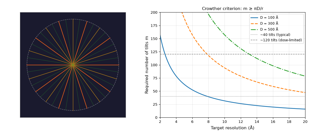
The right panel shows that for a typical 50 nm specimen, achieving 5 Å resolution would require ~300 tilts — far beyond what dose constraints allow. This fundamental tension between dose budget and Crowther sampling is a key driver for subtomogram averaging and denoising approaches in cryo-ET.
11.8. Iterative Reconstruction Methods#
Filtered backprojection is fast but treats each tilt image independently. Iterative methods improve reconstruction quality by treating it as an optimisation problem: find the 2D (or 3D) density that best explains all observed projections simultaneously.
SIRT (Simultaneous Iterative Reconstruction Technique): At each iteration, compute forward projections of the current estimate, compare with measured projections, backproject the residuals, and update the estimate. SIRT is more tolerant of the missing wedge and reduces the “star artifact” visible in FBP reconstructions.
Compressed sensing (CS) reconstruction: Biological structures are often sparse in an appropriate basis (e.g., sparse gradient). CS adds a regularisation term that promotes sparsity, enabling reasonable reconstruction quality even with very few tilt angles.
Deep learning methods: Neural networks can be trained to predict missing information or denoise tomograms. Self-supervised approaches exploit the even/odd frames of tilt movies to denoise each tilt image without requiring clean reference data.
11.9. Subtomogram Averaging#
Electron tomography preserves the 3D context of molecules in their native environment, but individual protein molecules within a tomogram are so small (\(\sim\)10–20 nm) and the SNR so low that single tomograms cannot reveal atomic detail. Subtomogram averaging (STA) combines the contextual information of tomography with the averaging power of SPA:
Template matching: A reference volume is cross-correlated with the tomogram in 3D to locate all candidate positions and orientations of a given complex.
Subtomogram extraction: Small 3D cubes (“subtomograms”) are extracted around each detected location.
Alignment and averaging: Subtomograms are aligned to each other using 3D cross-correlation and averaged, suppressing noise by \(\sqrt{N}\) as in SPA.
Classification: 3D classification can sort subtomograms by conformation, revealing structural heterogeneity.
STA achieves resolutions of 3–8 Å for large, abundant complexes in intact cells. The unique advantage over SPA is that the positions and orientations of the averaged copies are known in their cellular context — the distance distributions and lattice arrangements of molecular machines can be mapped directly.
11.10. Tilt Series Alignment and CTF Correction#
Before reconstruction, the tilt series images must be aligned to a common coordinate frame. Standard alignment uses fiducial markers — gold nanoparticles mixed into the sample before freezing, visible as high-contrast blobs in every tilt image. The 3D coordinates of the fiducials are refined by minimising reprojection errors across all tilts.
Fiducial-free alignment using cross-correlation of image patches is increasingly common and works well for data collected with good stage stability.
CTF correction in cryo-ET is more complex than in SPA because the defocus varies across a tilted specimen: a point at height \(h\) above the grid centre has defocus \(\Delta f + h \sin\theta\). CTF correction must therefore be applied locally, either per-tilt or per-sub-volume.
11.11. In-Situ Cryo-ET: Seeing Molecules in their Cellular Context#
The most powerful application of cryo-ET is imaging biological structures directly within the cell. In-situ cryo-ET can visualise organelles, cytoskeletal networks, membrane contacts, and macromolecular machines in the intact cellular environment, without the artefacts introduced by biochemical purification.
The main technical challenge is specimen thickness: whole mammalian cells (\(5\)–\(20\) µm thick) are far too thick for TEM. Solutions include:
Cryo-focused ion beam (cryo-FIB) milling: a focused ion beam sculpts a thin lamella (\(< 200\) nm) through the vitrified cell, exposing a thin slice suitable for TEM.
Cryo-sections: thin sections of high-pressure-frozen material, analogous to ultra-thin sectioning for conventional EM.
Cryo-FIB-SEM milling combined with cryo-ET and STA now routinely achieves sub-nanometre resolution of in-situ structures, making it possible to map entire interactomes within a cell volume.
11.12. References#
Avinash C. Kak and Malcolm Slaney. Principles of Computerized Tomographic Imaging. Society for Industrial and Applied Mathematics, Philadelphia, PA, 2001. doi:10.1137/1.9780898719277.