10. Random variables

Recommended reference: Wasserman [Was04], Sections 1.1–1.3, 2.1–2.2 and 3.1–3.3.

10.1. Introduction

A probability distribution assigns probabilities (real numbers in \([0,1]\)) to elements or subsets of a sample space. The elements of a sample space are called outcomes, subsets are called events.

The space of outcomes is usually of one of two kinds:

• some finite or countable set (modelling the number of particles hitting a detector, for example), or

• the real line, a higher-dimensional space or some subset of one of these (modelling the position of a particle, for example).

These correspond to the two types of probability distributions that are usually distinguished: discrete and continuous probability distributions.

10.2. Random variables

A random variable is any real-valued function on the space of outcomes of a probability distribution. Random variables can often be interpreted as observable (scalar) quantities such as length, position, energy, the number of occurrences of some event or the spin of an elementary particle.

Any random variable has a distribution function, which is how we usually describe random variables. We will look at distribution functions separately for discrete and continuous random variables.

10.3. Discrete random variables

A discrete random variable \(X\) can take finitely many or countably many distinct values \(x_0,x_1,x_2,\ldots\) in \(\RR\). It is characterised by its probability mass function (PMF).

Definition 10.1 (Probability mass function)

The probability mass function of the discrete random variable \(X\) is defined by

\[ f_X(x) = P(X = x). \]

One can visualise a probability mass function by placing a vertical bar of height \(f_X(x)\) at each value \(x\), as in Fig. 10.1.

Show code cell source Hide code cell source

from matplotlib import pyplot
from myst_nb import glue

fig, ax = pyplot.subplots()
for x, px in ((-0.2, 0.3), (0.4, 0.2), (0.7, 0.5)):
	ax.add_line(pyplot.Line2D((x, x), (0, px), linewidth=2))
ax.set_xbound(-0.3, 0.8)
ax.set_ybound(0, 0.6)
ax.set_xlabel('$x$')
ax.set_ylabel('$f(x)$')

glue("pmf", fig)

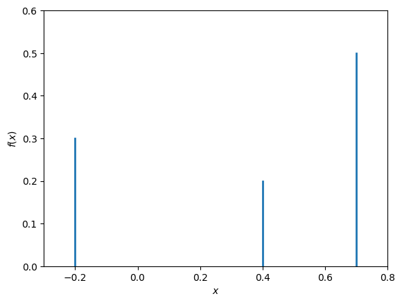
Fig. 10.1 Probability mass function of a discrete random variable.

Property 10.1 (Properties of a probability mass function)

Since the \(f_X(x)\) are probabilities, they satisfy

\[f_X(x) \in [0,1]\quad\text{for all }x\in\RR. \]

Since the \(x_i\) are all the possible values and their total probability equals 1, we also have

\[ \sum_{i=0}^\infty f_X(x_i) = 1. \]

10.4. Continuous random variables

For a continuous random variable \(X\), the set of possible values is usually a (finite or infinite) interval, and the probability of any single value occurring is usually zero. We therefore consider the probability of the value lying in some interval. This can be described by a probability density function (PDF).

Definition 10.2 (Probability density function)

The probability density function of the continuous random variable \(X\) is a function \(f_X\colon\RR\to\RR\) such that

\[ P(X\in[a,b]) = \int_a^b f_X(x) dx. \]

To visualise a continuous random variable, one often plots the probability density function, as in Fig. 10.2.

Property 10.2 (Properties of a probability density function)

• \(f_X(x)\ge0\) for all \(x\);

• \(\int_{-\infty}^\infty f(x)dx=1\).

Show code cell source Hide code cell source

from matplotlib import pyplot
from myst_nb import glue
import numpy as np

x = np.linspace(0, 16, 101)
fx = 1/120 * x**5 * np.exp(-x)

fig, ax = pyplot.subplots()
ax.plot(x, fx)
ax.set_xbound(0, 16)
ax.set_ybound(0, 0.2)
ax.set_xlabel('$x$')
ax.set_ylabel('$f(x)$')

glue("pdf", fig)

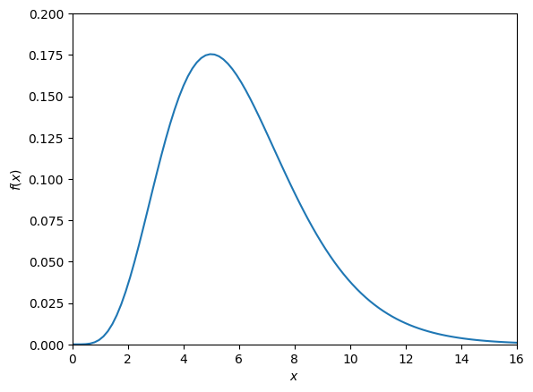
Fig. 10.2 Probability density function of a continuous random variable.

10.5. Expectation and variance

The expectation (or expected value, or mean) of a random variable is the average value of many samples. The variance and the closely related standard deviation measure by how much samples tend to deviate from the average.

Definition 10.3 (Expectation)

The expectation or mean of a discrete random variable \(X\) with probability mass function \(f_X\) is

\[ E(X) = \sum_x f_X(x) x = \sum_x P(X = x)x. \]

The expectation or mean of a continuous random variable \(X\) with probability density function \(f_X\) is

\[ E(X) = \int_{-\infty}^\infty x\,f_X(x) dx. \]

The expectation of \(X\) is often denoted by \(\mu\) or \(\mu(X)\).

Definition 10.4 (Variance and standard deviation)

The variance of a (discrete or continuous) random variable \(X\) with mean \(\mu\) is

\[ \Var(X) = E((X-\mu)^2). \]

The standard deviation of \(X\) is

\[ \sigma(X) = \sqrt{\Var(X)}. \]

It is not hard to show (see Exercise 10.3) that

(10.1)\[ \Var(X) = E(X^2) - E(X)^2. \]

10.6. Cumulative distribution functions

Besides the probability mass functions and probability density functions introduced above, it is often useful to look at cumulative distribution functions. Among other things, these have the advantage that the definition is the same for discrete and continuous random variables.

Definition 10.5 (Cumulative distribution function)

The cumulative distribution function of a (discrete or continuous) random variable \(X\) is the function \(F_X\colon\RR\to\RR\) defined by

\[ F_X(x) = P(X\le x). \]

If \(X\) is a discrete random variable, this comes down to

\[ F_X(x) = \sum_{y\le x} P(X=x). \]

This is illustrated in Fig. 10.3.

Show code cell source Hide code cell source

from matplotlib import pyplot
from myst_nb import glue

fig, ax = pyplot.subplots()
for x0, x1, h in ((-0.3, -0.2, 0.005), (-0.2, 0.4, 0.3),
                  (0.4, 0.7, 0.5), (0.7, 0.8, 0.995)):
    ax.add_line(pyplot.Line2D((x0, x1), (h, h), linewidth=2))

ax.set_xbound(-0.3, 0.8)
ax.set_ybound(0, 1)
ax.set_xlabel('$x$')
ax.set_ylabel('$F(x)$')

glue("cdf-discrete", fig)

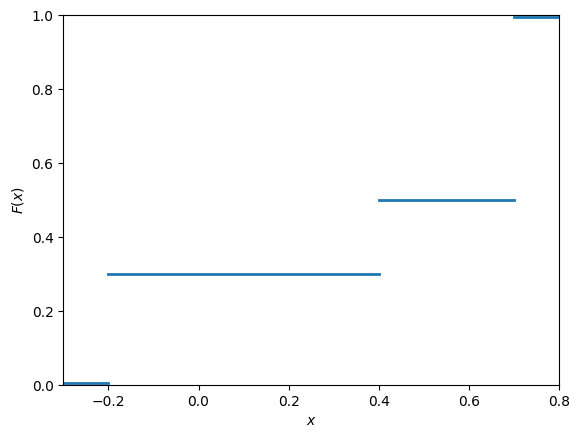
Fig. 10.3 Cumulative distribution function of the discrete random variable from Fig. 10.1.

Now suppose \(X\) is a continuous random variable. Taking the limit \(a\to-\infty\) in the definition of the probability density function, we obtain

\[ f_X(x) = P(X\le x) = \int_{-\infty}^x f_X(t) dt. \]

This is illustrated in Fig. 10.4.

Show code cell source Hide code cell source

from matplotlib import pyplot
from myst_nb import glue
import numpy as np

x = np.linspace(0, 16, 101)
Fx = 1 - 1/120 * (x**5 + 5*x**4 + 20*x**3 + 60*x**2 + 120*x + 120) * np.exp(-x)

fig, ax = pyplot.subplots()
ax.plot(x, Fx)
ax.set_xbound(0, 16)
ax.set_ybound(0, 1)
ax.set_xlabel('$x$')
ax.set_ylabel('$F(x)$')

glue("cdf", fig)

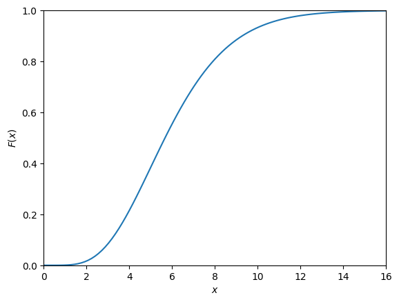
Fig. 10.4 Cumulative distribution function of the continuous random variable from Fig. 10.2.

10.7. Independence and conditional probability

Recommended reference for this subsection: Wasserman [Was04], Sections 2.5–2.8.

Informally speaking, two random variables \(X\) and \(Y\) are independent if knowledge of the value of one of the two does not tell us anything about the value of the other. However, knowledge of one random variable often does give you information about another random variable. This is encoded in the concept of conditional probability distributions.

To make the notions of indepence and conditional probability precise, we need two further concepts: the joint probability mass function \(P(X=x\text{ and }Y=y)\) in the case of discrete random variables, and the joint probability density function \(f_{X,Y}(x,y)\) in the case of continuous random variables. These describe the joint probability distribution of the two random variables \(X\) and \(Y\). Rather than defining these here, we refer to Wasserman [Was04], Section 2.5. We only note the relationship with the corresponding single-variable functions. If \(X\) and \(Y\) are discrete random variables, we have

\[ P(X = x) = \sum_y P(X = x\text{ and }Y=y) \quad\text{and}\quad P(Y = y) = \sum_x P(X = x\text{ and }Y=y). \]

Similary, if \(X\) and \(Y\) are continuous random variables, the relationship is given by

\[ f_X(x) = \int_{-\infty}^\infty f_{X,Y}(x,y)dy \quad\text{and}\quad f_Y(y) = \int_{-\infty}^\infty f_{X,Y}(x,y)dx. \]

In this situation, the distributions of \(X\) and \(Y\) individually are called the marginal distributions of the joint distribution of \(X\) and \(Y\).

Definition 10.6 (Independence of random variables)

Two discrete random variables \(X\) and \(Y\) are independent if for all possible values \(x\) and \(y\) of \(X\) and \(Y\), respectively, we have

\[ P(X=x\text{ and }Y=y) = P(X=x) P(Y=y). \]

Similarly, two continous random variables \(X\) and \(Y\) are independent if their probability density functions satisfy

\[ f_{X,Y}(x,y) = f_X(x) f_Y(y). \]

Definition 10.7 (Conditional probability)

Consider two discrete random variables \(X\) and \(Y\), and a value \(y\) such that \(P(Y=y)>0\). The conditional probability of \(x\) given \(y\) is defined as

\[ P(X=x\mid Y=y) = \frac{P(X=x\text{ and }Y=y)}{P(Y=y)}. \]

Analogously, consider two continuous random variables \(X\) and \(Y\), and a value \(y\) such that \(f_Y(y)>0\). The conditional probability of \(x\) given \(y\) is defined as

\[ f_{X\mid Y}(x\mid y) = \frac{f_{X,Y}(x,y)}{f_Y(y)}. \]

In Exercise 10.5, you will show that if two random variables \(X\) and \(Y\) are independent, then the distribution of \(X\) given a certain value of \(Y\) is the same as the distribution of \(X\).

10.8. Covariance and correlation

Recommended reference for this subsection: Wasserman [Was04], Section 3.3.

Definition 10.8 (Covariance of two random variables)

Let \(X\) and \(Y\) be random variables with means \(\mu_X\) and \(\mu_Y\), respectively. The covariance of \(X\) and \(Y\) is

\[ \Cov(X,Y) = E((X-\mu_X)(Y-\mu_Y)). \]

The correlation of \(X\) and \(Y\) is

\[ \rho(X,Y) = \frac{\Cov(X,Y)}{\sigma(X)\sigma(Y)}. \]

The covariance can be expressed in a way reminiscent of (10.1) as follows (see Exercise 10.6):

(10.2)\[ \Cov(X,Y) = E(XY)-E(X)E(Y). \]

Using the Cauchy–Schwarz inequality (see Exercise 8.4), one can show that the correlation satisfies \(-1\le\rho(X,Y)\le 1\).

10.9. Moments and the characteristic function

Note

The topics in this section are not necessarily treated in a BSc-level probability course. We include them both because they have applications in physics and data analysis, and because they connect nicely to various other topics in this module.

Definition 10.9 (Moments of a random variable)

Let \(X\) be a random variable. For \(j=0,1,\ldots\), the \(j\)-th moment of \(X\) is the expectation of \(X^j\).

Concretely, for a discrete random variable \(X\), this means that the \(j\)-th moment is given by

\[ E(X^j) = \sum_x x^j P(X=x). \]

For a continuous random variable, the \(j\)-th moment can be expressed as

\[ E(X^j) = \int_{-\infty}^\infty x^j f_X(x) dx. \]

Note that we have already encountered the first and second moments in the definition of the expectation (Definition 10.3) and in the formula (10.1) for the variance.

It is sometimes convenient to collect all the moments of \(X\) in a power series. For this, we include the moment generating function of \(X\).

Definition 10.10 (Moment generating function of a random variable)

Let \(X\) be a random variable. The moment generating function of \(X\) is the following function of a real variable \(t\):

\[ M_X(t) = E(\exp(tX)). \]

This definition may look a bit mysterious at first sight. Assuming that we can treat the random variable \(X\) in a similar way as an ordinary real number, we can compute the Taylor series of \(M_X(t)\) via the usual formula (see The exponential function), which will reveal how \(M_X(t)\) encodes the moments of \(X\):

\[\begin{split} \begin{aligned} M_X(t) &= E\left(\sum_{n=0}^\infty\frac{(tX)^n}{n!}\right)\\ &= \sum_{n=0}^\infty E\left(\frac{E((tX)^n)}{n!}\right)\\ &= \sum_{n=0}^\infty \frac{E(X^n)}{n!}t^n. \end{aligned} \end{split}\]

In some situations, it is better to use a variant called the characteristic function. (One reason is that the characteristic function is defined for every probability distribution; the moment generating function does not exist for ‘badly behaved’ distributions like the Cauchy distribution that we will see in Definition 11.1.)

Definition 10.11 (Characteristic function of a random variable)

Let \(X\) be a random variable. The characteristic function of \(X\) is the following (complex-valued) function of a real variable \(t\):

\[ \phi_X(t) = E(\exp(itX)). \]

A similar computation as above gives

\[ \phi_X(t) = \sum_{n=0}^\infty \frac{i^n E(X^n)}{n!}t^n. \]

On the other hand, using the probability density function \(f_X\), we can also express \(\phi_X(t)\) in a different way, namely as

\[ \phi_X(t) = \int_{-\infty}^\infty\exp(itx)f_X(x)dx. \]

This means that \(\phi_X(t)\) is essentially the Fourier transform of \(f_X\) (see Definition 3.1); more precisely, the relation is given by

\[ \phi_X(t) = \widehat{f_X}(-t/2\pi). \]

The characteristic function can be used to give a proof of the central limit theorem, which will be introduced in Section 12.3.

---

10.10. Exercises

Exercise 10.1

Show that the function

\[\begin{split} f(x) = \begin{cases} \displaystyle\frac{x^2}{30}& \text{if }x=1,2,3,4\\ 0& \text{otherwise} \end{cases} \end{split}\]

is a probability mass function.

Exercise 10.2

Which of the following functions are probability density functions?

1. \(f(x)=\begin{cases} 0& \text{if }x<0\\ x\exp(-x)& \text{if }x\ge 0\end{cases}\)

2. \(f(x)=\begin{cases} 1/4& \text{if }-2\le x\le 2\\ 0& \text{otherwise}\end{cases}\)

3. \(f(x)=\begin{cases} \frac{3}{4}(x^2-1)& \text{if }-2\le x\le 2\\ 0& \text{otherwise} \end{cases}\)

Exercise 10.3

Deduce (10.1) from the definition of the variance.

Exercise 10.4

Consider a continuous random variable \(X\) with probability density function

\[\begin{split} f(x)=\begin{cases} 0& \text{if }x<0,\\ \exp(-x)& \text{if }x\ge 0.\end{cases} \end{split}\]

Compute the expectation and the variance of \(X\).

Exercise 10.5

Consider two discrete random variables \(X\) and \(Y\). Show that if \(X\) and \(Y\) are independent, we have

\[ P(X=x\mid Y=y) = P(X=x)\quad \text{for all }x,y\text{ such that }P(Y=y)>0. \]

(Intuitively, this means that observing \(Y\) tells us nothing about the probability of observing a certain value of \(X\).)

Exercise 10.6

Let \(X\) and \(Y\) be random variables. Prove the formula (10.2).

Exercise 10.7

Show that the moment generating function of the random variable from Exercise 10.4 is given by

\[ M_X(t) = \frac{1}{1-t}. \]

Exercise 10.8

Let \(X\) be a random variable with moment generating function \(M_X(t)\). Show that for all \(n\ge0\), the \(n\)-th moment of \(X\) can be computed as the \(n\)-th derivative of \(M_X(t)\) at \(t=0\), i.e.

\[ E(X^n) = M_X^{(n)}(0). \]