2. Fourier series

The Fourier series of a function expresses the function as a linear combination of complex exponentials. This is extremely useful in many situations in mathematics, physics and engineering.

In terms of linear algebra, the theory of Fourier series provides an orthonormal basis for the Hilbert space of square-integrable functions on the interval \([0,1]\); see also Hilbert spaces and operators.

2.1. Definition and basic properties

Definition 2.1 (Fourier series)

Let \(f\) be a (real or complex) function on the interval \([0,1]\). The Fourier series of \(f\) is the infinite series

\[ \sum_{n=-\infty}^\infty c_n \exp(2\pi i n x) \]

where the complex numbers \(c_n\) are defined by

\[ c_n = \int_0^1 f(x)\exp(-2\pi i n x)dx. \]

We call these \(c_n\) the Fourier coefficients of \(f\).

One reason why Fourier series are useful is that the basis functions

\[ e_n(x) = \exp(2\pi i n x) \]

form an orthonormal system: in Exercise 2.1, you will show that these functions satisfy

\[\begin{split} \int_0^1 e_m(x)\overline{e_n(x)}dx = \begin{cases} 1& \text{if }m=n,\\ 0& \text{if }m\ne n. \end{cases} \end{split}\]

(See also Example 8.6 in the section on Hilbert spaces and operators.)

There are also other ways of writing this series, namely via Euler’s formula

\[ \exp(i x)=\cos x + i\sin x \]

or the equivalent form

\[\begin{split} \begin{aligned} \cos x &= \frac{\exp(ix)+\exp(-ix)}{2},\\ \sin x &= \frac{\exp(ix)-\exp(-ix)}{2i}. \end{aligned} \end{split}\]

In particular, for functions \(f\) satisfying \(f(1-x)=f(x)\) this gives rise to Fourier cosine series

\[ f(x) = \sum_{n=0}^\infty a_n \cos(2\pi n x) \]

and for functions \(f\) satisfying \(f(1-x)=-f(x)\) to Fourier sine series

\[ f(x) = \sum_{n=1}^\infty b_n \sin(2\pi n x); \]

see Exercise 2.4 for details.

One can show that if \(f\) is continuous, then the Fourier series of \(f\) converges to \(f\) at every point. For an example where \(f\) is discontinuous, see Exercise 2.2.

2.2. Examples

2.2.1. The Fourier series of a sawtooth function

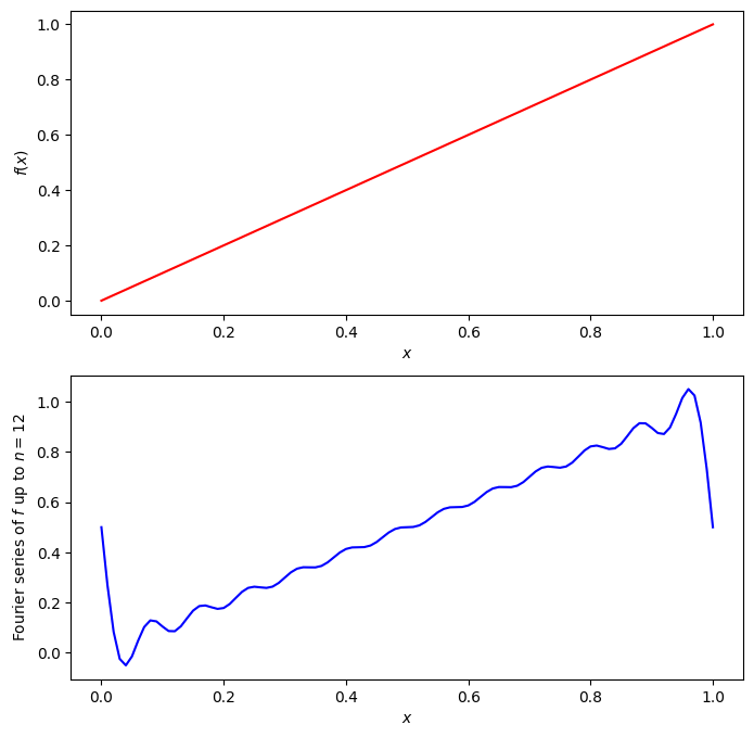
Consider the function \(f(x)=x\) on the interval \([0,1]\). To find its Fourier series, we compute the integrals defining the coefficients \(c_n\) for all integers \(n\). We have

\[ c_0 = \int_0^1 x dx = \frac{1}{2}. \]

For \(n\ne0\) we compute \(c_n\) using integration by parts:

\[\begin{split} \begin{aligned} c_n &= \int_0^1 x\exp(-2\pi i n x)dx\\ &= \left.-\frac{1}{2\pi i n}x\exp(-2\pi i n x)\right|_{x=0}^1 +\frac{1}{2\pi i n}\int_0^1\exp(-2\pi i n x)dx\\ &= \left(-\frac{1}{2\pi i n}+0\right)+0\\ &= -\frac{1}{2\pi i n}. \end{aligned} \end{split}\]

We conclude that the Fourier series of \(f\) is

\[ \frac{1}{2}-\sum_{n\ne0}\frac{1}{2\pi i n}\exp(2\pi i n x), \]

where the sum ranges over all non-zero integers \(n\). Combining the terms corresponding to \(n\) and \(-n\) and using the identity

\[ -\frac{1}{2\pi i n}\exp(2\pi i n x) + \frac{1}{2\pi i n}\exp(2\pi i (-n) x) = -\frac{1}{\pi n}\sin(2\pi n x), \]

we can simplify this to

\[ \frac{1}{2}-\sum_{n=1}^\infty\frac{1}{\pi n}\sin(2\pi n x), \]

Show code cell source Hide code cell source

from matplotlib import pyplot as plot
from myst_nb import glue
import numpy as np

fig, ax = plot.subplots(2, 1, figsize=(8,8))

x = np.linspace(0, 1, 101)

ax[0].plot(x, x, color='red')
ax[0].set_xlabel('$x$')
ax[0].set_ylabel('$f(x)$')

f_appr = 1/2 - sum((np.sin(2*np.pi*n*x)/(np.pi*n) for n in range(1, 13)), 0*x)
ax[1].plot(x, f_appr, color='blue')
ax[1].set_xlabel('$x$')
ax[1].set_ylabel('Fourier series of $f$ up to $n=12$')

glue("sawtooth", fig, display=False)

Fig. 2.1 A sawtooth function and an approximation to its Fourier series

2.2.2. The Fourier series of a half-wave rectified sine function

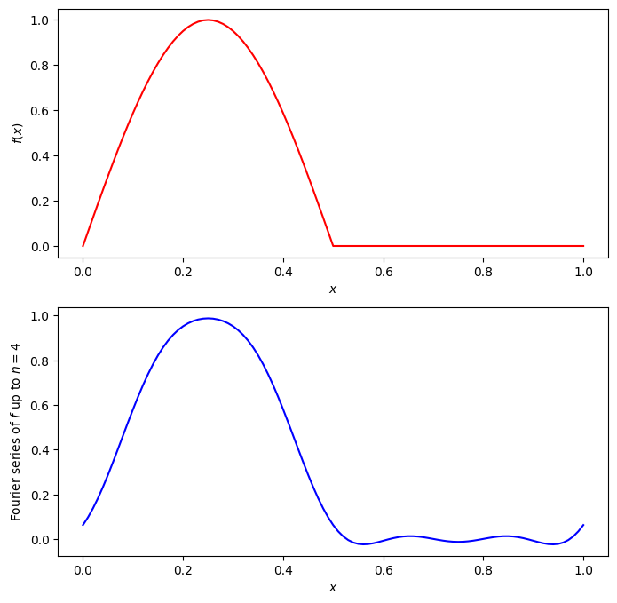
Consider the half-wave rectified sine function

(2.1)\[\begin{split} f(x) = \begin{cases} \sin(2\pi x)& \text{if }0\le x\le 1/2,\\ 0& \text{if }1/2<x\le 1. \end{cases} \end{split}\]

In Exercise 2.3, you will show that the Fourier coefficients are given by

(2.2)\[\begin{split} \begin{aligned} c_1 &= \frac{1}{4i},\quad c_{-1}=-\frac{1}{4i},\\ c_n &= 0\text{ for $n\ne\pm1$ odd},\\ c_n &= -\frac{1}{\pi(n^2-1)}\quad\text{for $n$ even}. \end{aligned} \end{split}\]

Show code cell source Hide code cell source

from matplotlib import pyplot as plot
from myst_nb import glue
from numpy import linspace, sin, cos, heaviside, pi

fig, ax = plot.subplots(2, 1, figsize=(8,8))

x = linspace(0, 1, 101)

ax[0].plot(x, sin(2*pi*x) * heaviside(0.5-x, 0.5), color='red')
ax[0].set_xlabel('$x$')
ax[0].set_ylabel('$f(x)$')

f_appr = 1/pi + 1/2*sin(2*pi*x) - 2/pi * sum((1/((2*n)**2-1)*cos(2*pi*(2*n)*x) for n in range(1, 3)), 0*x)
ax[1].plot(x, f_appr, color='blue')
ax[1].set_xlabel('$x$')
ax[1].set_ylabel('Fourier series of $f$ up to $n=4$')

glue("rectified-sine", fig, display=False)

Fig. 2.2 A half-wave rectified sine function and an approximation to its Fourier series

---

2.3. Exercises

Exercise 2.1

Prove the orthogonality relation

\[\begin{split} \int_0^1 e_m(x)\overline{e_n(x)}dx = \begin{cases} 1& \text{if }m=n,\\ 0& \text{if }m\ne n \end{cases} \end{split}\]

where

\[ e_n(x) = \exp(2\pi i n x). \]

Exercise 2.2

Consider the function \(f\) on the interval \([0,1]\) defined by

\[\begin{split} f(x) = \begin{cases} 1& \text{if }0\le x\le 1/2,\\ 0& \text{if }1/2<x\le 1. \end{cases} \end{split}\]

1. Compute the Fourier series of \(f\).

2. Compute the value of this Fourier series at \(x=1/2\).

Exercise 2.3

Consider the the half-wave rectified sine function \(f\) defined by (2.1).

1. Prove the formula (2.2) for the Fourier coefficients of \(f\).

2. Show that the Fourier series of \(f\) can be rewritten as

   \[ f(x) = \frac{1}{\pi} + \frac{1}{2}\sin(2\pi x) - \frac{2}{\pi} \sum_{n>0\text{ even}} \frac{1}{n^2-1}\cos(2\pi nx). \]

Exercise 2.4

Consider a complex-valued function \(f\) on the interval \([0,1]\) with Fourier series

\[ f(x)=\sum_{n=-\infty}^\infty c_n\exp(2\pi i nx). \]

1. Show that \(f\) can be written as a Fourier cosine series if and only if \(f(1-x)=f(x)\).

2. Show that \(f\) can be written as a Fourier sine series if and only if \(f(1-x)=-f(x)\).