11. Basic probability distributions

Recommended reference: Wasserman [Was04], in particular Sections 2.3 and 2.4.

In this section we cover some of the most important examples of probability distributions.

11.1. Discrete probability distributions

11.1.1. Discrete uniform distribution

The idea of the uniform distribution is that there is a finite collection of possible outcomes, each of which is equally likely.

The discrete uniform distribution on a set \(S\) of size \(n\) (for example the set \(\{1,2,\ldots,n\}\)) assigns probability \(1/n\) to each element of \(S\):

\[ P(X = x) = \frac{1}{n}\quad(x\in S). \]

Show code cell source Hide code cell source

from matplotlib import pyplot
from myst_nb import glue

fig, ax = pyplot.subplots()
for x in (1, 2, 3, 4):
	ax.add_line(pyplot.Line2D((x, x), (0, 0.25), linewidth=2))
ax.set_xbound(0, 5)
ax.set_ybound(0, 0.3)
ax.set_xlabel('$x$')
ax.set_ylabel('$f(x)$')

glue("discrete-uniform", fig)

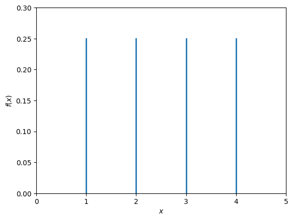
Fig. 11.1 Probability mass function of a uniform discrete random variable with values \(1,2,3,4\).

11.1.2. Bernoulli distribution

The Bernoulli distribution models an experiment that can have two outcomes, for example a (possibly biased) coin flip. We will denote the two possible outcomes by \(0\) and \(1\). The distribution depends on a parameter \(p\in[0,1]\), which is by definition the probability that the outcome equals 1. We have

\[ P(X = 0) = 1-p\quad\text{and}\quad P(X = 1) = p. \]

Show code cell source Hide code cell source

from matplotlib import pyplot
from myst_nb import glue

fig, ax = pyplot.subplots()
for x, px in ((0, 0.3), (1, 0.7)):
	ax.add_line(pyplot.Line2D((x, x), (0, px), linewidth=2))
ax.set_xbound(-.5, 1.5)
ax.set_ybound(0, 0.8)
ax.set_xlabel('$x$')
ax.set_ylabel('$f(x)$')

glue("bernoulli", fig)

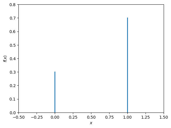
Fig. 11.2 Probability mass function of a Bernoulli random variable with \(p=0.7\).

11.1.3. Binomial distribution

The binomial distribution with parameters \(n\) and \(p\) is defined by the probability mass function

\[ P(X = k) = \binom{n}{k} p^k(1-p)^{n-k}. \]

Here \(\binom{n}{k}=\frac{n!}{k!(n-k)!}\) is the usual binomial coefficient.

This can be viewed as a sum of \(n\) Bernoulli random variables with parameter \(p\).

Show code cell source Hide code cell source

from math import comb
from matplotlib import pyplot
from myst_nb import glue

fig, ax = pyplot.subplots()
n = 10
p = 0.7
for k in range(n + 1):
	pk = comb(n, k) * p**k * (1 - p)**(n - k)
	ax.add_line(pyplot.Line2D((k, k), (0, pk), linewidth=2))
ax.set_xbound(-1, n+1)
ax.set_ybound(0, 0.3)
ax.set_xlabel('$x$')
ax.set_ylabel('$f(x)$')

glue("binomial", fig)

Fig. 11.3 Probability mass function of a binomial random variable with parameters \(n=10\) and \(p=0.7\).

11.1.4. Poisson distribution

The Poisson distribution with rate \(\lambda\) is defined by the probability mass function

\[ P(X = k) = \exp(-\lambda)\frac{\lambda^k}{k!}. \]

Note

The total probability equals 1 because of the Taylor series expansion of the exponential function, which tells us that

\[ \sum_{k=0}^\infty\frac{\lambda^k}{k!} = \exp(\lambda); \]

see The exponential function.

The Poisson distribution is used to model situations where we have a series of independent random events that occur with some fixed rate in a given time interval.

(See also the section on the exponential distribution below.)

Show code cell source Hide code cell source

from math import exp, factorial
from matplotlib import pyplot
from myst_nb import glue

fig, ax = pyplot.subplots()
L = 2
for k in range(10):
	pk = exp(-L) * L**k / factorial(k)
	ax.add_line(pyplot.Line2D((k, k), (0, pk), linewidth=2))
ax.set_xbound(-1, 11)
ax.set_ybound(0, 0.3)
ax.set_xlabel('$x$')
ax.set_ylabel('$f(x)$')

glue("poisson", fig)

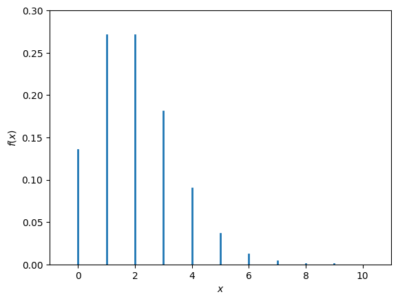
Fig. 11.4 Probability mass function of a Poisson random variable with parameter \(\lambda=2\).

11.2. Continuous probability distributions

11.2.1. Continuous uniform distribution

This a continuous analogue of the discrete uniform distribution described above. In this case, the intuition that “all outcomes are equally likely” is strictly speaking meaningless, since every outcome has probability 0.

The continuous uniform distribution on a bounded interval \([a,b]\) has constant probability density function \(1/(b-a)\) on the interval:

\[ f(x) = \frac{1}{b-a}\quad(a\le x\le b). \]

Show code cell source Hide code cell source

from matplotlib import pyplot
from myst_nb import glue

fig, ax = pyplot.subplots()
ax.plot((-2, -1, -1, 3, 3, 4), (0, 0, 1/4, 1/4, 0, 0))
ax.set_xbound(-2, 4)
ax.set_ybound(0, 0.3)
ax.set_xlabel('$x$')
ax.set_ylabel('$f(x)$')

glue("continuous-uniform", fig)

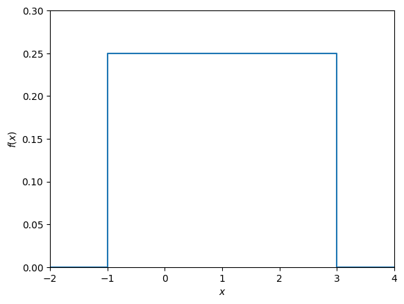
Fig. 11.5 Probability density function of a uniform continuous random variable.

11.2.2. Normal or Gaussian distribution

The normal or Gaussian distribution with mean \(\mu\) and variance \(\sigma^2\) is defined by the probability density function

\[ f(x) = \frac{1}{\sigma\sqrt{2\pi}} \exp\biggl(-\frac{(x-\mu)^2}{2\sigma^2}\biggr)\quad(x\in\RR). \]

The normal distribution with mean \(0\) and variance \(1\) is also called the standard normal distribution.

The normal distribution is one of the most common probability distributions. One of the reasons for this is the role that it plays in the Central limit theorem.

Show code cell source Hide code cell source

from matplotlib import pyplot
from myst_nb import glue
import numpy as np

x = np.linspace(-2, 2, 101)
fx = np.exp(-np.pi * x**2)

fig, ax = pyplot.subplots()
ax.plot(x, fx)
ax.set_xbound(-2, 2)
ax.set_ybound(0, 1.2)
ax.set_xlabel('$x$')
ax.set_ylabel('$f(x)$')

glue("gaussian", fig)

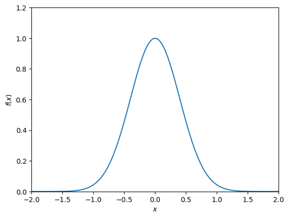
Fig. 11.6 Probability density function of a normal (Gaussian) random variable with mean \(0\) and variance \(\frac{1}{2\pi}\).

11.2.3. Exponential distribution

The exponential distribution with rate \(\lambda>0\) is defined by the probability density function

\[ f(x) = \lambda\exp(-\lambda x)\quad(x\ge0). \]

Show code cell source Hide code cell source

from matplotlib import pyplot
from myst_nb import glue
import numpy as np

x = np.linspace(0, 4, 101)
fx = np.exp(-x)

fig, ax = pyplot.subplots()
ax.plot(x, fx)
ax.set_xbound(0, 4)
ax.set_ybound(0, 1.2)
ax.set_xlabel('$x$')
ax.set_ylabel('$f(x)$')

glue("exponential", fig)

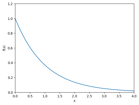
Fig. 11.7 Probability density function of an exponential random variable.

11.2.4. Cauchy or Lorentz distribution

We include this example mostly to illustrate that seemingly nice probability distributions can display “pathological” behaviour.

Definition 11.1 (Cauchy distribution)

The Cauchy (or Lorentz) distribution is defined by the probability density function

\[ f(x) = \frac{1}{\pi(1+x^2)}. \]

The graph of this function (see figure below) looks a bit like that of a normal distribution, but the ‘tails’ decrease much less rapidly.

Let us see what happens if we try to calculate the expectation of this distribution:

\[\begin{split} \begin{aligned} E(X) &= \int_{-\infty}^\infty xf(x)dx\\ &=\frac{1}{\pi}\int_{-\infty}^\infty \frac{x}{1+x^2}dx\\ &=\frac{1}{\pi}\cdot\biggl.\frac{1}{2}\log(x^2+1)\biggr|_{x=-\infty}^\infty\\ &=\infty-\infty \end{aligned} \end{split}\]

This shows that the expectation is undefined. The same holds for the variance.

Show code cell source Hide code cell source

from matplotlib import pyplot
from myst_nb import glue
import numpy as np

x = np.linspace(-4, 4, 101)
fx = 1 / (np.pi * (1 + x**2))

fig, ax = pyplot.subplots()
ax.plot(x, fx)
ax.set_xbound(-4, 4)
ax.set_ybound(0, .4)
ax.set_xlabel('$x$')
ax.set_ylabel('$f(x)$')

glue("cauchy", fig)

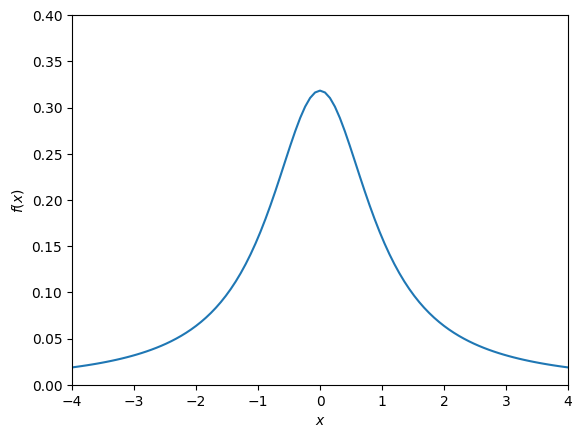
Fig. 11.8 Probability density function of a Cauchy (Lorentz) random variable.

---

11.3. Exercises

Exercise 11.1

Calculate the expectation and variance of a Bernoulli distribution with parameter \(p\).

Exercise 11.2

Check that the total probability of a binomial distribution with parameters \(n\) and \(p\) equals 1 (as it should).

Exercise 11.3

Calculate the expectation and variance of the continuous uniform distribution on the interval \([-1,3]\).

Exercise 11.4

Check that the total probability of a normal distribution with mean \(\mu\) and variance \(\sigma^2\) equals 1 (as it should).

Hint: use the Gaussian integral (3.3).

Exercise 11.5

Suppose \(X_1\) and \(X_2\) are independent continuous random variables, where \(X_1\) follows the uniform distribution on \([0,1]\) and \(X_2\) follows the uniform distribution on \([0,2]\). Find the probability density function for the random variable \(Z = X_1 + X_2\).