3. Fourier transforms

Like Fourier series, the Fourier transform of a function \(f\) is a way to decompose \(f\) into complex exponentials. This is a very useful tool in quantum mechanics and signal processing, for example.

The difference between Fourier series and Fourier transforms is that while Fourier series are defined for functions on a bounded interval (or equivalently for periodic functions), the Fourier transform can be applied to functions on the whole real line. As a consequence, all complex exponentials

\[ e_t(x)=\exp(itx) \]

for arbitrary real numbers \(t\) are needed to decompose arbitrary functions \(f\) as above.

3.1. Definition and basic properties

Definition 3.1 (Fourier transform)

Let \(f\) be a (real or complex) function on the real line \(\mathbb{R}\). The Fourier transform of \(f\) is the function

(3.1)\[ \hat f(y) = \int_{-\infty}^\infty f(x)\exp(-2\pi i x y)dx. \]

Warning

Various other conventions exist for the definition of the Fourier transform, so be careful when combining different sources.

The most important property is that using the Fourier transform \(\hat f\), we can express the original function \(f\) using a very similar formula.

Theorem 3.1 (Fourier inversion formula)

Let \(f\) be a (real or complex) function on the real line \(\mathbb{R}\). Then we can recover \(f\) from its Fourier transform \(\hat f\) via the formula

\[ f(x) = \int_{-\infty}^\infty \hat f(y)\exp(2\pi i x y)dy. \]

This means that \(\hat f\) describes the ‘coefficients’ that occur when expressing \(f\) as a ‘linear combination’ of exponential functions, except the expression involves an integral rather than a sum.

Property 3.1 (Properties of the Fourier transform)

Here are several other properties of the Fourier transform, for a given function \(f\) with Fourier transform \(\hat f\):

1. For any real number \(a\), the Fourier transform of \(f(x-a)\) equals \(\exp(-2\pi i ay)\hat f(y)\).

2. For any real number \(a\ne0\), the Fourier transform of \(f(ax)\) equals \(|a|^{-1}\hat f(y/a)\).

3. The Fourier transform of \(\frac{df}{dx}\) is \(2\pi iy\hat f(y)\).

4. The Fourier transform of \(xf(x)\) is \(\frac{1}{2\pi i y}\) times the Fourier transform of \(\frac{df}{dx}\).

5. (Plancherel’s theorem) We have

   \[ \int_{-\infty}^\infty|f(x)|^2 dx= \int_{-\infty}^\infty|\hat f(y)|^2 dy. \]

The first four of these properties are fairly direct consequences of the definition of the Fourier transform. The last property is more difficult to show; see Exercise 3.2.

3.2. Examples

3.2.1. The Fourier transform of a rectangular function

Consider the rectangular (or “square pulse”) function

(3.2)\[\begin{split} f(x) = \begin{cases} 1& \text{if }-1/2\le x\le 1/2,\\ 0& \text{otherwise} \end{cases} \end{split}\]

(see Fig. 3.1 below). We compute

\[\begin{split} \begin{aligned} \hat f(y) &= \int_{-1}^1 \exp(-2\pi i x y)dx\\ &= \left[-\frac{1}{2\pi i y}\exp(-2\pi i x y)\right]_{x=-1/2}^{1/2}\\ &= -\frac{1}{2\pi i y}(\exp(-\pi i y)-\exp(\pi i y)). \end{aligned} \end{split}\]

Using the formula

\[ \sin t = \frac{e^{it}-e^{-it}}{2i} \]

we obtain

\[ \hat f(y) = \sinc y, \]

where the \(\sinc\) function is defined by

\[ \sinc(t) = \frac{\sin(\pi t)}{\pi t}. \]

Show code cell source Hide code cell source

from matplotlib import pyplot as plot
from myst_nb import glue
import numpy as np

fig, ax = plot.subplots(2, 1, figsize=(8,8))

ax[0].plot((-1, -.5, -.5, .5, .5, 1), (0, 0, 1, 1, 0, 0), color='red')
ax[0].set_xlabel('$x$')
ax[0].set_ylabel('$f(x)$')

y = np.linspace(-4, 4, 101)
fhat = np.sinc(y)
ax[1].plot(y, fhat, color='blue')
ax[1].set_xlabel('$y$')
ax[1].set_ylabel('$\\hat f(y)$')

glue("rectangular", fig, display=False)

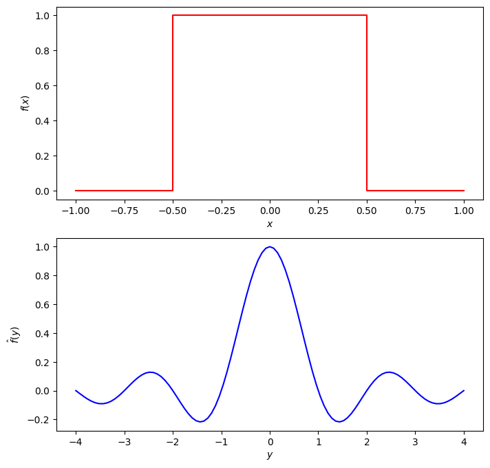
Fig. 3.1 A rectangular function and its Fourier transform

3.2.2. The Fourier transform of a Gaussian function

For a fixed \(a>0\), consider the function

\[ f(x) = \exp(-\pi ax^2) \]

(see Fig. 3.2 below). We compute

\[\begin{split} \begin{aligned} \hat f(y) &= \int_{-\infty}^\infty \exp(-\pi a x^2-2\pi i x y)dx\\ &= \int_{-\infty}^\infty \exp(-\pi a(x-iy/a)^2 - \pi y^2/a)dx\\ &= \int_{-\infty}^\infty \exp(-\pi a(x-iy/a)^2)dx\cdot \exp(- \pi y^2/a). \end{aligned} \end{split}\]

To finish the computation, we need the contour integration technique from complex analysis. The integral in the above expression can be interpreted as the integral of the function \(\exp(-\pi z^2)\) over the line \(\Im z=-y/a\). Shifting the line of integration to \(\Im z=0\) (the real axis), we get

\[ \hat f(y) = \int_{-\infty}^\infty \exp(-\pi ax^2)dx\cdot \exp(- \pi y^2/a). \]

Finally, we make use of the Gaussian integral

(3.3)\[ \int_{-\infty}^\infty \exp(-\pi ax^2)dx = a^{-1/2} \]

(if you don’t know this, look it up in your favourite reference for integrals) to conclude

\[ \hat f(y) = a^{-1/2} \exp(-\pi y^2/a). \]

Show code cell source Hide code cell source

from matplotlib import pyplot as plot
from myst_nb import glue
import numpy as np

fig, ax = plot.subplots(2, 1, figsize=(8,8))
a = 0.5

x = np.linspace(-2, 2, 101)
f = np.exp(-np.pi * a * x**2)
ax[0].plot(x, f, color='red')
ax[0].set_xlabel('$x$')
ax[0].set_ylabel('$f(x)$')

y = np.linspace(-2, 2, 101)
fhat = a**(-1/2) * np.exp(-np.pi / a * y**2)
ax[1].plot(y, fhat, color='blue')
ax[1].set_xlabel('$y$')
ax[1].set_ylabel('$\\hat f(y)$')

glue("gaussian", fig, display=False)

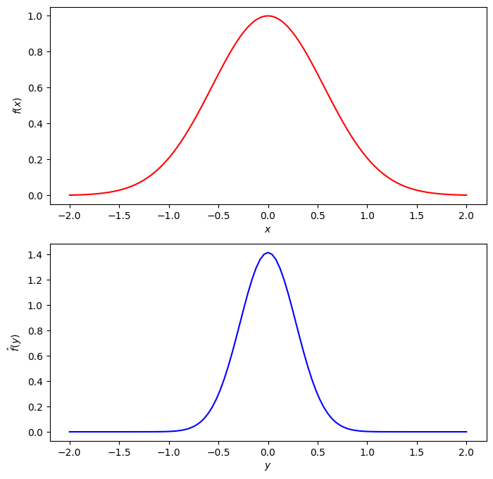
Fig. 3.2 The Gaussian function \(f_{1/2}(x)\) and its Fourier transform \(\widehat{f_{1/2}}(y)=\sqrt{2}f_2(y)\)

3.3. Fourier transforms and convolutions

The convolution of two functions is an operation that has applications in many areas, such as physics, engineering and probability. We briefly introduce it here because of an interesting and useful relation between convolutions and the Fourier transform: the Fourier transform converts convolution into (pointwise) multiplication. This is made precise by Theorem 3.2 below.

Definition 3.2 (Convolution)

Let \(f\) and \(g\) be (real or complex) functions on the real line \(\mathbb{R}\). The convolution of \(f\) and \(g\) is the function \(f * g\) defined by

(3.4)\[ (f * g)(y) = \int_{-\infty}^\infty f(x)g(y - x)dx. \]

Theorem 3.2 (Fourier transform and convolution)

Let \(f\) and \(g\) be (real or complex) functions on the real line \(\mathbb{R}\). Then the Fourier transform of the convolution of \(f\) and \(g\) equals the (pointwise) product of the Fourier transforms:

\[ \widehat{f * g}(z) = \hat f(z) \hat g(z). \]

Proof. We compute the Fourier transform of \(f * g\) by interchanging the order of integration and using part 1 of Property 3.1 for the function \(g(y-x)\):

\[\begin{split} \begin{aligned} \widehat{f * g}(z) &= \int_{-\infty}^\infty \int_{-\infty}^\infty f(x)g(y - x)dx\, \exp(-2\pi i yz)dy\\ &= \int_{-\infty}^\infty f(x) \left(\int_{-\infty}^\infty g(y - x)\exp(-2\pi i yz)dy\right)dx\\ &= \int_{-\infty}^\infty f(x)\left(\exp(-2\pi i xz)\hat g(z)\right)dx\\ &= \hat f(z)\hat g(z). \end{aligned} \end{split}\]

Symmetrically, the Fourier transform converts a pointwise product into a convolution; see Exercise 3.5.

---

3.4. Exercises

Exercise 3.1

For a fixed \(a>0\), compute the Fourier transform of the function

\[ f(x) = \exp(-a|x|). \]

Exercise 3.2

Do Problem 2.20 in Griffiths [Gri95], which gives a step-by-step derivation of the Fourier inversion formula (called Plancherel’s theorem in [Gri95]).

Exercise 3.3

Consider the rectangular function \(f\) defined by (3.2). Show that the convolution of \(f\) with itself equals the ‘triangular’ function \(\Lambda\) (sketch the graph!) given by

(3.5)\[\begin{split} \Lambda(x) = \begin{cases} 1+x& \text{if }-1\le x\le 0\\ 1-x& \text{if }0\le x\le 1\\ 0& \text{if }|x|\ge 1. \end{cases} \end{split}\]

Exercise 3.4

Use the previous exercise and Theorem 3.2 to compute the Fourier transform of the triangular function \(\Lambda\) defined by (3.5).

Exercise 3.5

Show that if \(f\) and \(g\) are two functions on the real line, then the following analogue of Theorem 3.2 holds:

\[ (\hat f * \hat g)(z) = \widehat{fg}(z). \]

Hint: use the Fourier inversion formula.