12. Central limit theorem

Recommended reference: Wasserman [Was04], Sections 5.3–5.4.

The central limit theorem is a very important result in probability theory. It tell us that when we have \(n\) independent and identically distributed random variables, the distribution of their average (up to suitable shifting and rescaling) approximates a normal distribution as \(n\to\infty\).

12.1. Sample mean

Consider a sequence of independent random variables \(X_1, X_2, \ldots\) distributed according to the same distribution function (which can be discrete or continuous). We say \(X_1, X_2, \ldots\) are independent and identically distributed (or i.i.d.).

Note

For a precise definition of independence of random variables, see Section 2.9 in Wasserman [Was04].

Definition 12.1

The \(n\)-th sample mean of \(X_1,X_2,\ldots\) is

\[ \overline{X}_n = \frac{1}{n}\sum_{i=1}^n X_i. \]

Note that \(\overline{X}_n\) is itself again a random variable.

12.2. The law of large numbers

As above, consider i.i.d. samples \(X_1, X_2, \ldots\), say with distribution function \(f\). We assume that \(f\) has finite mean \(\mu\). The law of large numbers says that the \(n\)-th sample average is likely to be close to \(\mu\) for sufficiently large \(n\).

Theorem 12.1 (Law of large numbers)

For every \(\epsilon>0\), the probability

\[ P(|\overline{X}_n-\mu|>\epsilon) \]

tends to \(0\) as \(n\to\infty\).

Note

The above formulation is known as the weak law of large numbers; there are also stronger versions, but the differences are not important here.

The figure below illustrates the law of large numbers for the average of the first \(n\) out of 1000 dice rolls.

Show code cell source Hide code cell source

import numpy as np
from matplotlib import pyplot
from myst_nb import glue

rng = np.random.default_rng()
N = 1000
n = np.arange(1, N + 1, 1)
X = rng.integers(1, 7, N)
Xbar = np.cumsum(X) / n

fig, ax = pyplot.subplots()
ax.plot((0, 1000), (3.5, 3.5))
ax.plot(n, Xbar)

ax.set_xlabel('$n$')
ax.set_ylabel('$\\overline{X}_n$')

glue("lln", fig)

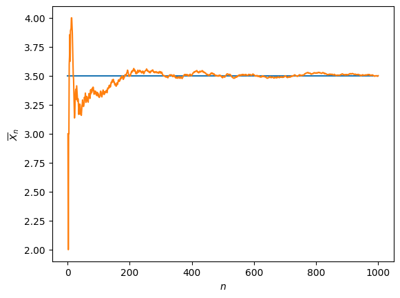
Fig. 12.1 Illustration of the law of large numbers: average of \(n\) dice rolls as \(n\to\infty\).

Warning

If the mean of the distribution function \(f\) does not exist, then the law of large numbers is meaningless. This is illustrated for the Cauchy distribution (see Definition 11.1) in the figure below.

Show code cell source Hide code cell source

import numpy as np
from matplotlib import pyplot
from myst_nb import glue

rng = np.random.default_rng(seed=37)
N = 1000
n = np.arange(1, N + 1, 1)
X = rng.standard_cauchy(N)
Xbar = np.cumsum(X) / n

fig, ax = pyplot.subplots()
ax.plot((0, 1000), (0, 0))
ax.plot(n, Xbar)

ax.set_xlabel('$n$')
ax.set_ylabel('$\\overline{X}_n$')

glue("lln-cauchy", fig)

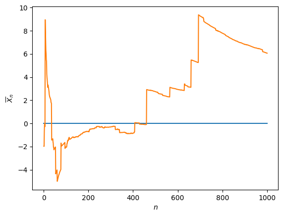
Fig. 12.2 Failure of the law of large numbers: average of \(n\) samples from the Cauchy distribution as \(n\to\infty\).

12.3. The central limit theorem

Again, we consider a sequence of i.i.d. samples \(X_1, X_2, \ldots\) with distribution function \(f\). We assume \(f\) has finite mean \(\mu\) and variance \(\sigma^2\).

By the law of large numbers, the shifted sample mean

\[ \overline{X}_n-\mu = \frac{1}{n}(X_1+\cdots+X_n)-\mu \]

has expectation 0.

Theorem 12.2 (Central limit theorem)

The distribution of the sequence of random variables

\[ Y_n = \frac{\sqrt{n}}{\sigma}(\overline{X}_n-\mu) \]

converges to the standard normal distribution as \(n\to\infty\).

Roughly speaking, we can write this as

\[ \overline{X}_n \approx \mu + \frac{\sigma}{\sqrt{n}}Z \]

where \(Z\) is a random variable following a standard normal distribution, or as

\[ \overline{X}_n \longrightarrow \mathcal{N}\biggl(\mu,\frac{\sigma}{\sqrt{n}}\biggr) \quad\text{as }n\to\infty, \]

where \(\mathcal{N}(\mu,\sigma)\) denotes the normal distribution with mean \(\mu\) and standard deviation \(\sigma\).

Show code cell source Hide code cell source

# Adapted from
# https://furnstahl.github.io/Physics-8820/notebooks/Basics/visualization_of_CLT.html
# by Dick Furnstahl (license: CC BY-NC 4.0)

from math import comb, factorial
import numpy as np

from matplotlib import pyplot
from myst_nb import glue

# Mean and standard deviation of our distribution
mu = 0.5
sigma = 1 / np.sqrt(12)

def bates_pdf(x, n):
    # https://en.wikipedia.org/wiki/Bates_distribution
    return (n / (2 * factorial(n - 1)) *
            sum((-1)**k * comb(n, k) * (n*x - k)**(n-1) * np.sign(n*x - k) for k in range(n + 1)))

def normal_pdf(x, mu, sigma):
    return (1/(np.sqrt(2*np.pi) * sigma) *
            np.exp(-((x - mu)/sigma)**2 / 2))

def plot_ax(ax, n):
    """
    Plot the n-th sample mean and the limiting normal distribution.
    """
    sigma_tilde = sigma / np.sqrt(n)
    x_min = mu - 4*sigma_tilde
    x_max = mu + 4*sigma_tilde

    ax.set_title('$n={}$'.format(n))
    ax.set_xlabel('$x$')
    ax.set_ylabel('$f(x)$')
    ax.set_xlim(x_min, x_max)

    # plot a normal pdf with the same mu and sigma
    # divided by the sqrt of the sample size.
    x_pts = np.linspace(x_min, x_max, 200)
    y_pts = normal_pdf(x_pts, mu, sigma_tilde)
    z_pts = bates_pdf(x_pts, n)
    ax.plot(x_pts, y_pts, color='gray')
    ax.plot(x_pts, z_pts)

sample_sizes = [1, 2, 3, 4, 8, 16]

# Plot a series of graphs to show the approach to a Gaussian.
fig, axes = pyplot.subplots(3, 2, figsize=(8, 8))

for ax, n in zip(axes.flatten(), sample_sizes):
    plot_ax(ax, n)

fig.tight_layout(w_pad=1.8)

glue("clt", fig)

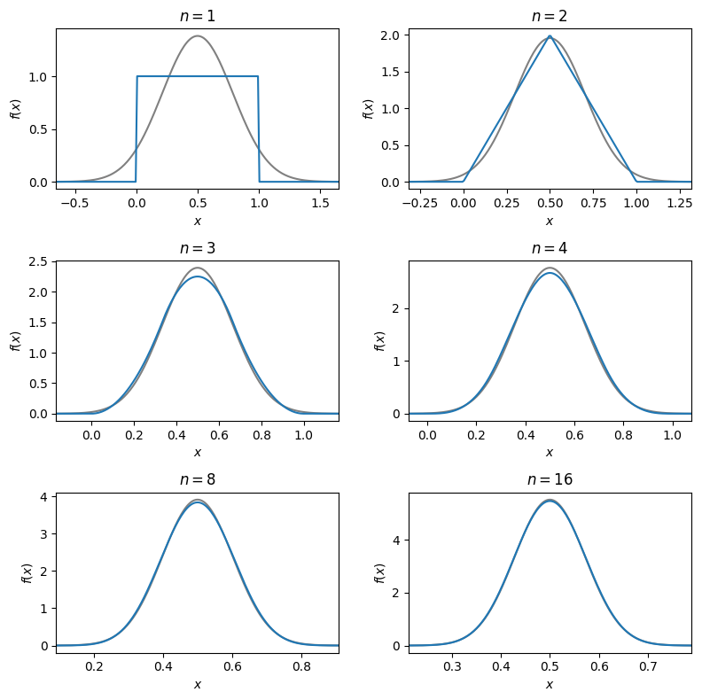
Fig. 12.3 Illustration of the central limit theorem for an average of \(n\) uniformly random samples

Show code cell source Hide code cell source

from math import comb, factorial
import numpy as np

from matplotlib import pyplot
from myst_nb import glue

p = 0.7

# Mean and standard deviation of our distribution
mu = p
sigma = np.sqrt(p*(1 - p))

def binomial_pmf(k, n):
    return comb(n, k) * p**k * (1 - p)**(n - k)

def normal_pdf(x, mu, sigma):
    return (1/(np.sqrt(2*np.pi) * sigma) *
            np.exp(-((x - mu)/sigma)**2 / 2))

def plot_ax(ax, n):
    """
    Plot a histogram on axis ax that shows the distribution of the
    n-th sample mean.  Add the limiting normal distribution.
    """
    sigma_tilde = sigma / np.sqrt(n)
    x_min = mu - 4*sigma_tilde
    x_max = mu + 4*sigma_tilde

    ax.set_title('$n={}$'.format(n))
    ax.set_xlabel('$x$')
    ax.set_ylabel('$f(x)$')
    ax.set_xlim(x_min, x_max)

    # plot a normal pdf with the same mu and sigma
    # divided by the sqrt of the sample size.
    x_pts = np.linspace(x_min, x_max, 200)
    y_pts = normal_pdf(x_pts, mu, sigma_tilde)
    ax.plot(x_pts, y_pts, color='gray')
    for k in range(n + 1):
        ax.add_line(pyplot.Line2D((k/n, k/n), (0, n * binomial_pmf(k, n)),
                    linewidth=2))

sample_sizes = [1, 2, 4, 8, 16, 32]

# Plot a series of graphs to show the approach to a Gaussian.
fig, axes = pyplot.subplots(3, 2, figsize=(8, 8))

for ax, n in zip(axes.flatten(), sample_sizes):
    plot_ax(ax, n)

fig.tight_layout(w_pad=1.8)

glue("clt-bern", fig)

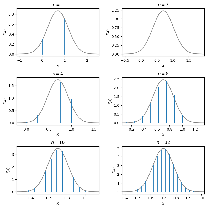
Fig. 12.4 Illustration of the central limit theorem for an average of \(n\) Bernoulli random samples (probability mass function scaled by a factor \(n\) for comparison with the probability density function of the normal distribution)

---

12.4. Exercises

Exercise 12.1

Suppose a certain species of tree has average height of 20 metres with a standard deviation of 3 metres. A dendrologist measures 100 of these trees and determines their average height. What will the mean and standard deviation of this average height be?

Exercise 12.2

Suppose \(X\) and \(Y\) are two independent continuous random variables which follow the standard normal distribution \(\mathcal{N}(0,1)\). In whatever programming language you like, compute and plot a histogram of \(n\) samples from \(X+Y\) for \(n = 100,1000,\) and \(10000\). What can you conclude about the random variable \(X+Y\)? Repeat the same exercise, but this time with \(X/Y\). What can you conclude about the random variable \(X/Y\)? Think about the central limit theorem as you explain your reasoning.