14. Differential equations#
A common form of models explaining physical, economical, or biological phenomena are those that relate to one or more unknown functions and their derivatives (rates of change). These equations are called differential equations and are often very difficult or impossible to be solved in a closed form. However, numerical solutions will allow us to use these equations for designing engineering models and systems.
14.1. Ordinary differential equations#
An ordinary differential equation (ODE) is an equation containing an unknown function of only one variable \(y(x)\), its derivatives \(y',..., y^{n}\), and some given functions of \(x\). The term “ordinary” is used in contrast to the term “partial differential equation”, which may be with respect to more than one independent variable. Here is an example of an ODE of order \(n\):
\(a_n(x) y^{(n)} + a_{n-1}(x) y^{(n-1)} + \cdots + a_1(x) y' + a_0(x) y_0 = f(x)\)
14.2. Euler’s method and first-order equations#
Euler’s method is the simplest numerical method for approximating solutions of differential equations. Consider the first-order equation below:
\(y' = f(y,x) \ , \ \ y(x_0)=y_0\)
The linear approximation of \(y(t_{n+1})\) using the Euler formula is:
\(y(x_{n+1}) = y(x_{n})+f(y,x)(x_{n+1}-x_{n})\)
Therefore, to find the values of the function \(y\) at all \(x_n\), given \(y_0\) and \(f(y,x)\), we can start with finding \(y(x_{1})\) using the Euler’s formula and repeat the process through a for loop for \(y(x_{2}),y(x_{3}),...\).
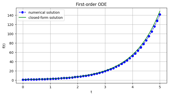
14.2.1. Example#
Approximate and plot solutions of \(\frac{dy}{dt} = e^{t} \ , \ \ y(0)=1\), using Euler’s formula for \(t\in[0,5]\) at evenly spaced grid points of size \(h=0.1\). Hint: the closed form solution is \(y(t)=e^t\).
import numpy as np
import matplotlib.pyplot as plt

# Define parameters
h = 0.1
t = np.arange(0, 5+h, h) # Numerical grid
f = lambda y,t: np.exp(t)
y0 = 1

# Explicit Euler Method
y = np.zeros(len(t))
y[0] = y0

for i in range(0, len(t) - 1):
    y[i + 1] = y[i] + h*f(y[i],t[i])

plt.figure(figsize = (8, 4))
plt.plot(t, y, 'bo--', label='numerical solution')
plt.plot(t, np.exp(t), 'g', label='closed-form solution')
plt.title('First-order ODE')
plt.xlabel('t')
plt.ylabel('f(t)')
plt.grid()
plt.legend(loc='upper left')
plt.show()
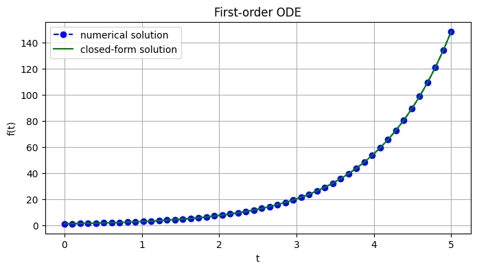
14.3. Solving ODEs with SciPy#
You can also use scipy.integrate.odeint(func, y0, t) to find the solution of a first-order ODE, where func=\(y'\), y0 is the initial condition, and t includes the time points at which the solution should be reported. The example below uses this function to find an approximate solution for \(\frac{df}{dt} = e^{t} \ , \ \ f(0)=1\).
import numpy as np
from scipy.integrate import odeint
import matplotlib.pyplot as plt

# parameters
t = np.linspace(0,5)
f = lambda y,t: np.exp(t)
y0 = 1

# solve ODE
y = odeint(f,y0,t)

# plot results
plt.figure(figsize = (8, 4))
plt.plot(t, y, 'bo--', label='numerical solution')
plt.plot(t, np.exp(t), 'g', label='closed-form solution')
plt.title('First-order ODE')
plt.xlabel('t')
plt.ylabel('f(t)')
plt.grid()
plt.legend(loc='upper left')
plt.show()
14.4. Higher-order ODEs and order reduction#
Most numerical solutions can only solve first-order equations. Therefore, to solve higher-order differential equations using these methods we first need to rewrite them as first-order equations. Let’s see how we can do this order reduction by applying it to the second-order equation shown below:
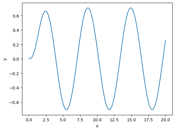
\(y''+2y'+3y=2sin(x)\) or \(\frac{d^2y}{dx^2}+2\frac{dy}{dx}+3y=2sin(x)\)
This second-order equation can be rewriten as two first-order equations by:
First, we introduce two new independent variables to replace \(y'\), and \(y\) as: \(u_1=y'\), and \( u_0=y\). Note that, we don’t need to introduce a new variable for \(y''\) (the highest-order derivative).
Next, we need to find the first-order equations for \(u'_1\), and \( u'_0\): \(y'=u_1 → u_0'=u_1 \\ y''=2sin(x)-2y'-3y → u'_1=2sin(x)-2u_1-3u_0\)
We can now write this ODE in a matrix form: \( u'=\begin{bmatrix} u'_0 \\ u'_1\end{bmatrix} =\begin{bmatrix} u_1 \\ 2sin(x)-2u_1-3u_0\end{bmatrix}=f(u,x)\).
Python implementation: We can now use odeint to solve the second-order equation above with \(y'_0=0\), and \(y_0=0\):
import numpy as np
from scipy.integrate import odeint
import matplotlib.pyplot as plt

def dudx(u, x):
    return [u[1], -2*u[1] - 3*u[0] + 2*np.sin(x)]

u0 = [0, 0]
xs = np.linspace(0, 20, 200)
us = odeint(dudx, u0, xs)
ys = us[:,0]

plt.xlabel("x")
plt.ylabel("y")
plt.plot(xs,ys);
14.5. Example 1:#
This assignment is dapted from Problem 7.37 in Fundamentals of Electric Circuits (Alexander & Sadiku, 2017).
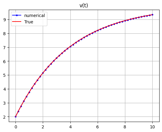
A circuit is described by \(4\frac{dv}{dt}+v=10\), with \(v_0=2 V\). Find \(v(t)\) for \(t>=0\). Note that the closed form solution is \(v(t)=10-8 e ^{-t/4}\)
Solution: we can rewrite this equation as \(\frac{dv}{dt}=-\frac{1}{4}v-\frac{10}{4}\), therefore \(f(v,t)=-\frac{1}{4}v-\frac{10}{4}\)
ts = np.linspace(0,10,51)
v0 = 2
f = lambda v,t: -v/4+2.5


ys = odeint(f,v0,ts)
ys_true = 10-8*np.exp(-ts/4)

plt.plot(ts,ys,'b.-',ts,ys_true,'r-')
plt.legend(['numerical','True'])
plt.grid(True)
plt.title("v(t)")
plt.show()
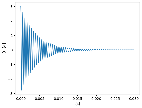
14.6. Example 2:#
This assignment is dapted from example 8.6 in Fundamentals of Electric Circuits (Alexander & Sadiku, 2017).
A series RLC circuit is described by \(L \frac{d^2i}{dt^2} + R \frac{di}{dt} + \frac{1}{C}i = 0\), where \(L = 8 m H\), \(R = 4 Ω\), and \(C = 1\mu F\). Find \(i(t)\) for \(t>=0\) with \(i_0 = 3 A\), \(di_0/dt= 0\).
Solution: Since this is a second-order ODE, we first introduce: \(u_0=i\), and \(u_1=di/dt\).
\( U'=\begin{bmatrix} u'_0 \\ u'_1\end{bmatrix} =\begin{bmatrix} u_1 \\ - \frac{R}{L} u_1 -\frac{1}{RC}u_0 \end{bmatrix}=f(u,t)\)
import numpy as np
from scipy.integrate import odeint
import matplotlib.pyplot as plt

R=4
L=8e-3
C=1e-6

def f(u, x):
    return [u[1], -(R/L)*u[1] - (1/(L*C))*u[0] + 0]

u0 = [3.0, 0.0]
ts = np.linspace(0.0, 0.03, 10**6)
us = odeint(f, u0, ts)
ys = us[:,0]

# this is also the closed loop response
# ys_true=np.exp(-250*ts)*(3*np.cos(11180*ts)+0.0671*np.sin(11180*ts))

plt.xlabel("t[s]")
plt.ylabel("i(t) [A]")
plt.plot(ts,ys);