Trees

3.8. Trees#

Recursion is often used with linked data structures. A linked data structure is a type of data structure constructed by linking several objects of the same type together with pointers. In this section we will take a look at one of the most common recursive data structures in computer science: trees.

3.8.1. Nomenclature of trees#

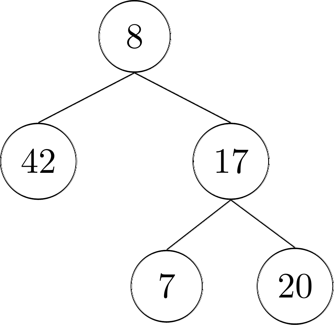
Trees in the mathematical world are often drawn in the opposite direction compared to real-world trees, with the root of the tree at the top. Why? Maybe because most people write from top of page downwards. The root has zero or more children nodes that each form the root of a subtree. Consider for example the following tree:

Nodes are represented by circles. The nodes of a tree can contain any type of data, but we will in this example each node contains an integer.

The node containing \(8\) is the root of this tree, with \(42\) and \(17\) being its children. Both \(42\) and \(17\) are root of subtrees. For example, the subtree rooted in \(17\) has three nodes: \(17\) as the root with its children \(7\) and \(20\).

Nodes with no children are called leaf nodes. In our example tree, the leaf nodes are \(42\), \(7\) and \(20\).

We will formalise this structure—trees—when we learn about sets and relations in the next chapter, but for now we will settle for the following informal definition:

Definition 3.1 (Tree node (informal))

A node in a tree has a) a value, b) a list of nodes.

There are many more names used in a description of a tree, and some of these might vary a bit between textbooks. In this book, we use the following set of terminology. Notice how some of these are recursively defined!

Parent of \(x\): The node in whose list of nodes \(x\) occurs.
Siblings of \(x\): The other nodes in the list of children of \(x\)’s parent.
Descendants of \(x\): \(x\) and the descendants of the children of \(x\).
Ancestors of \(x\): \(x\) and the ancestors of the parent of \(x\).
Leaf: A node that has no children.
Root: The node that has no parent.
Binary tree: A tree where every node has at most 2 children.
Height: The largest number of vertices on a path from a leaf to the root, excluding the leaf.

Using this terminology, we can now say that the example tree above has a height of 2, contains 3 leaves, and is a binary tree. Further, the ancestors of \(20\) are \(20\) itself, \(17\) and \(8\).

3.8.2. An application of trees#

Trees are popular in computer science because they can be used for a large number of different applications, from sorting, to memory management and keeping track of family members (though the latter is not strictly speaking a tree: do you see why?). During the course Algorithms & Data Structures you will encounter many of these applications as well. Trees are a special type of a more general linked data structure, graphs, which are also very useful in computer science. We’ll look at graphs in the next chapter.

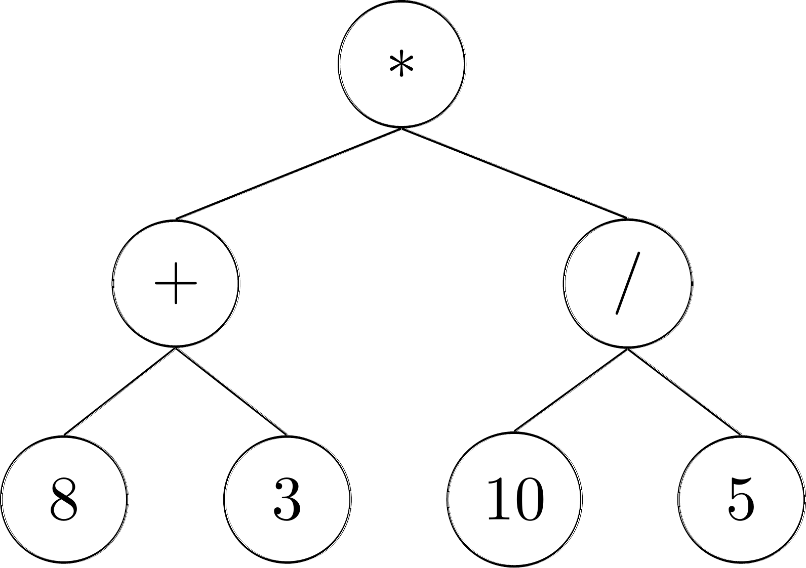
For now we will only take a look at one example, using trees to represent mathematical formulae. Consider for example the expression: \((8+3) * (10 / 5)\). We can represent this using a tree, by having every operator be the root of a subtree, and the leaves of the tree be the different numbers:

Notice how this tree has different types of ‘data’ in its nodes: some are numbers and some are operators.

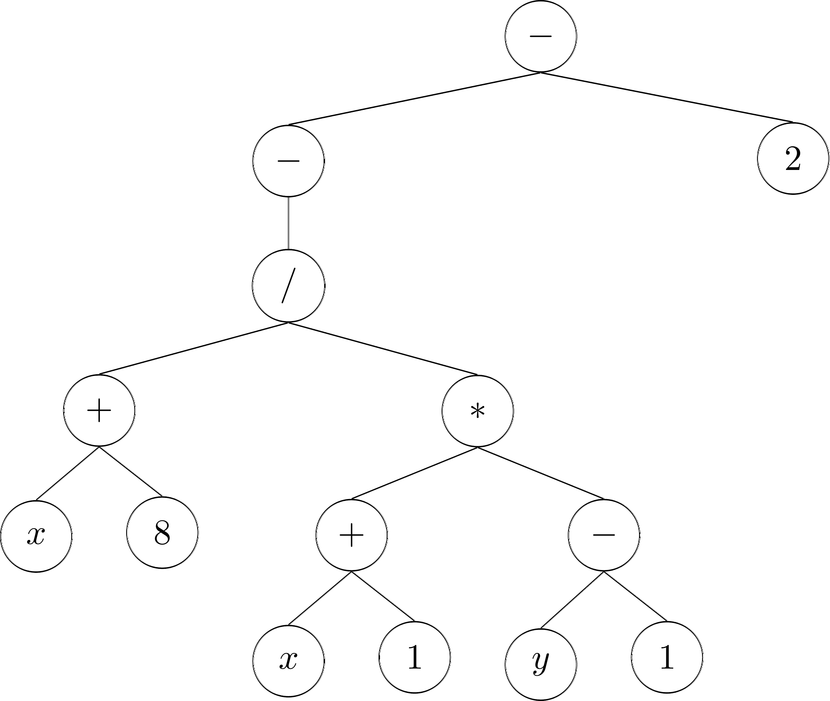
You will find that for each of these trees there is exactly one expression that matches it! For example, the following tree represents the statement: \(-\frac{x+8}{(x+1)(y-1)} - 2\)

If you already have some programming experience, perhaps you can already see how this could be a useful way to represent mathematical expressions. We can now write a recursive algorithm that first evaluates the value of the children, and then applies the operator at the root of the subtree. Simply put:

If this node is a number, return the number.
Else evaluate the value of each child.
Combine the values using the operator in this node.

In the exercises you will practice also with turning statements from propositional and predicate logic into trees.

3.8.3. Binary trees in Java*#

For an example of recursive definitions and proof by induction, we’ll look at the data structure known as a binary tree. As you can guess from its name, and as we indicated earlier, a binary tree is a type of tree.

Warning

If you don’t already know about objects and pointers, you will not be able to follow the rest of this section. Time to read about it on the internet?

Like any tree, a binary tree consists of nodes linked together in a tree-like structure. A binary tree can be empty, or it can consist of a node (the root of the tree) and two smaller binary trees (called the left subtree and the right subtree of the tree). You can already see the recursive structure: a tree can contain smaller trees. Notice that this recursive definition immediately limits each node to have at most two children.

In the programming language Java, the nodes of a tree can be represented by objects belonging to this class

class BinaryTreeNode {
	int item;   // An integer value stored in the node.
	BinaryTreeNode left;   // Pointer to left subtree.
	BinaryTreeNode right;  // Pointer to right subtree.
}

An empty tree is represented by a pointer that has the special value null. If root is a pointer to the root node of a tree, then root.left is a pointer to the left subtree and root.right is a pointer to the right subtree. Of course, both root.left and root.right can be null if the corresponding subtree is empty. Similarly, root.item is a name for the integer in the root node.

Let’s say that we want a function that will find the sum of all the integers in all the nodes of a binary tree. We can do this with a simple recursive function. The base case of the recursion is an empty tree. Since there are no integers in an empty tree, the sum of the integers in an empty tree is zero. For a non-empty tree, we can use recursion to find the sums of the integers in the left and right subtrees, and then add those sums to the integer in the root node of the tree. In Java, this can be expressed as follows:

int TreeSum( BinaryTreeNode root ) {
	// Find the sum of all the integers in the
	// tree that has the given root.
	int answer;
	if (root == null) {
	  // The tree is empty.
		answer = 0;
	} else {
			answer = TreeSum(root.left);
			answer += TreeSum(root.right);
			answer += root.item;
	}
	return answer;
}

We can use the second form of the principle of mathematical induction to prove that this function is correct.

Theorem 3.13

The function TreeSum, defined above, correctly computes the sum of all the integers in a binary tree.

Proof. We use induction on the number of nodes in the tree. Let \(P(n)\) be the statement ‘’TreeSum correctly computes the sum of the nodes in any binary tree that contains exactly \(n\) nodes’’. We show that \(P(n)\) is true for every natural number \(n\).

Consider the case \(n=0\). A tree with zero nodes is empty, and an empty tree is represented by a null pointer. In this case, the if statement in the definition of TreeSum assigns the value 0 to the answer, and this is the correct sum for an empty tree. So, \(P(0)\) is true.

Let \(k\) be an arbitrary natural number, with \(k>0\). Suppose we already know \(P(x)\) for each natural number \(x\) with \(0\le x < k\). That is, TreeSum correctly computes the sum of all the integers in any tree that has fewer than \(k\) nodes. We must show that it follows that \(P(k)\) is true, that is, that TreeSum works for a tree with \(k\) nodes. Suppose that root is a pointer to the root node of a tree that has a total of \(k\) nodes. Since the root node counts as a node, that leaves a total of \(k-1\) nodes for the left and right subtrees, so each subtree must contain fewer than \(k\) nodes. By the induction hypothesis, we know that TreeSum(root.left) correctly computes the sum of all the integers in the left subtree, and TreeSum(root.right) correctly computes the sum of all the integers in the right subtree. The sum of all the integers in the tree is root.item plus the sums of the integers in the subtrees, and this is the value computed by TreeSum. So, TreeSum does work for a tree with \(k\) nodes. This completes the induction.

□

Note how closely the structure of the inductive proof follows the structure of the recursive function. In particular, the second principle of mathematical induction is very natural here, since the size of subtree could be anything up to one less than the size of the complete tree. It would be very difficult to use the first principle of induction in a proof about binary trees.

3.8.4. Exercises#

Exercise (1)

Draw a binary tree so that the root has a total of 8 descendants, and there is node that has exactly 4 ancestors.

Exercise (2)

What is the value of the expression represented by the following tree?

Exercise (3)

Draw a tree for the propositional logic statement: \((p \wedge q) \rightarrow \lnot(r \leftrightarrow z)\)

Exercise (4)

Draw a tree for the predicate logic statement: \(\forall x (P(x) \rightarrow (Q(x) \vee \exists y (R(x,y))))\)

Exercise (5)

A leaf node in a binary tree is a node in which both the left and the right subtrees are empty. Prove that the following recursive function correctly counts the number of leaves in a binary tree:

int LeafCount(BinaryTreeNode root) {
	// Counts the number of leaf nodes in
	// the tree with the specified root.
	int count;
	if (root == null) {
		count = 0;
	} else if (root.left == null && root.right == null) {
		count = 1;
	} else {
		count = LeafCount(root.left);
		count += LeafCount(root.right);
	}
	return count;
}

Exercise (6)

A binary search tree satisfies the following property: If node is a pointer to any node in the tree, then all the integers in the left subtree of node are less than node.item and all the integers in the right subtree of node are greater than or equal to node.item. Prove that the following recursive subroutine prints all the integers in a binary search tree in non-decreasing order:

void SortPrint(BinaryTreeNode root) {
	// Assume that root is a pointer to the
	// root node of a binary sort tree.  This 
	// subroutine prints the integers in the
	// tree in non-decreasing order.
	if (root == null) {
		// There is nothing to print.
	}
	else {
		SortPrint(root.left);
		System.out.println(root.item);
		SortPrint(root.right);
	}
}

Exercise (7)

Extend Theorem 3.13 to work for non-binary trees.