8.2. Quadratic forms

8.2.1. Introduction and terminology

The simplest functions from \(\R^n\) to \(\R\) are linear functions

\[ f(x_1,\ldots,x_n) = \sum_{i=1}^n a_ix_i +b \, =\, a_1x_1 + a_2x_2 + \cdots + a_nx_n + b. \]

In short \(f(\mathbf{x}) = \mathbf{a}^T\mathbf{x} + b\), for some vector \(\mathbf{a}\) in \(\R^n\) and some number \(b\) in \(\R\).

This is the common notion of linearity in calculus. To be linear in the linear algebra sense the constant term \(b\) must be zero.

After that come the quadratic functions

(8.2.1)\[q(x_1,\ldots,x_n) = \sum_{i,j=1}^{n} a_{ij}x_ix_j + \sum_{i=1}^{n} b_ix_i + c,\]

where all parameters \(a_{ij}\), \(b_i\) and \(c\) are real numbers.

A quadratic function in the two variables \(x_1\), \(x_2\) thus becomes

\[ q(x_1,x_2) = a_{11}x_1^2 + a_{12}x_1x_2 + a_{21}x_2x_1 + a_{22}x_2^2 + b_1x_1 + b_2x_2 + c, \]

Note that this can be written as

\[\begin{split} q(x_1,x_2) = \begin{pmatrix} x_1 & x_2 \end{pmatrix} \begin{pmatrix} a_{11} & a_{12} \\ a_{21} & a_{22} \end{pmatrix}\begin{pmatrix} x_1 \\ x_2 \end{pmatrix} + \begin{pmatrix} b_1 & b_2 \end{pmatrix}\begin{pmatrix} x_1 \\ x_2 \end{pmatrix} + c. \end{split}\]

In general, a shorthand representation of Equation (8.2.1) becomes

\[ q(\mathbf{x}) = \mathbf{x}^TA\mathbf{x} + \mathbf{b}^T\mathbf{x} + c, \]

for an \(n\times n\)-matrix \(A\), a vector \(\vect{b}\) in \(\R^n\), and a number \(c\) in \(\R\).

The part \(\mathbf{x}^TA\mathbf{x}\) is called a quadratic form.

Example 8.2.1

For the matrix \(A = \begin{pmatrix} 1 & 2 \\ 4 & 3 \end{pmatrix}\) the corresponding quadratic form is

\[\begin{split} \begin{array}{rcl} q(\vect{x}) = \begin{pmatrix} x_1 & x_2 \end{pmatrix} \begin{pmatrix} 1 & 2 \\ 4& 5 \end{pmatrix}\begin{pmatrix} x_1 \\ x_2 \end{pmatrix} &=& \begin{pmatrix} x_1 & x_2 \end{pmatrix} \begin{pmatrix} x_1 + 2x_2 \\ 4x_1+ 5x_2 \end{pmatrix} \\ &=& x_1^2 + (2+4)x_1x_2 + 5x_2^2 \\ &=& x_1^2 + 6x_1x_2 + 5x_2^2. \end{array} \end{split}\]

Note that the last expression does not uniquely determine the matrix. We can split the coefficient \(6\) of the term \(x_1x_2\) in a different way and will end up with a different matrix. If we distribute it evenly over \(x_1x_2\) and \(x_2x_1\) we get a symmetric matrix.

\[\begin{split} \begin{array}{rcl} x_1^2 + 6x_1x_2 + 5x_2^2 &=& x_1^2 + (3+3)x_1x_2 + 5x_2^2 \\ &=& x_1^2 + 3x_1x_2 + 3x_2x_1 + 5x_2^2 \\ &=& x_1(x_1 + 3x_2) + x_2(3x_1 + 5x_2) \\ &=& \begin{pmatrix} x_1 & x_2 \end{pmatrix} \begin{pmatrix} x_1 + 3x_2 \\ 3x_1+ 5x_2 \end{pmatrix}\\ &=&\begin{pmatrix} x_1 & x_2 \end{pmatrix} \begin{pmatrix} 1 & 3 \\ 3 & 5 \end{pmatrix}\begin{pmatrix} x_1 \\ x_2 \end{pmatrix}. \end{array} \end{split}\]

The above example leads to the first proposition about quadratic forms.

Proposition 8.2.1

Every quadratic form \(q(\mathbf{x})\) can be written uniquely as

\[ q(\mathbf{x}) = \mathbf{x}^TA\mathbf{x} \]

for a symmetric matrix \(A\).

This symmetric matrix \(A\) is then called the matrix of the quadratic form.

Example 8.2.2

We will find the symmetric matrix \(A\) for the symmetric form

\[ q(x_1,x_2,x_3) = x_1^2 + 2x_2^2 + 5 x_3^2 - 4 x_1x_2 + 6 x_2x_3. \]

So we need a symmetric matrix \(A = \begin{pmatrix} a_{11} & a_{12} & a_{13} \\ a_{12} & a_{22} & a_{23} \\ a_{13} & a_{23} & a_{33} \end{pmatrix}\).

From

\[ \mathbf{x}^TA\mathbf{x} = a_{11}x_1^2 + a_{22}x_2^2 + a_{33}x_3^2 + 2a_{12}x_1x_2 + 2a_{13}x_1x_3 + 2a_{23}x_2x_3 \]

we read off

\[ a_{11} = 1, \, a_{22} = 2, \, a_{33} = 5, \,\,\text{and}\,\, a_{12} = -2, \, a_{13} = 0, \, a_{23} = 3. \]

So \(A = \begin{pmatrix} 1 & -2 & 0 \\ -2 & 2 & 3 \\ 0 & 3 & 5 \end{pmatrix}\).

If we restrict ourselves to two variables, we see that the graph of a linear function \(z = a_1x_1 + a_2x_2 + b\) is a plane.

Fig. 8.2.1 The plane \(z = \frac13x_1 - x_2 +2\).

The graph of a quadratic function is a curved surface. Figure 8.2.2 and Figure 8.2.3 show two of these quadratic surfaces.

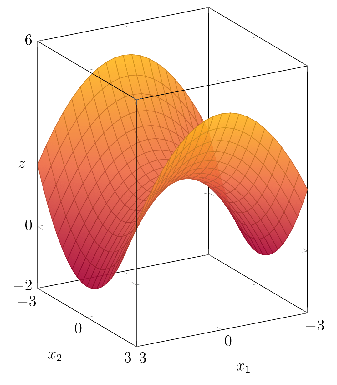
Fig. 8.2.2 The surface \(z = -\frac13x_1^2 + \frac13x_2^2 + 2 \).

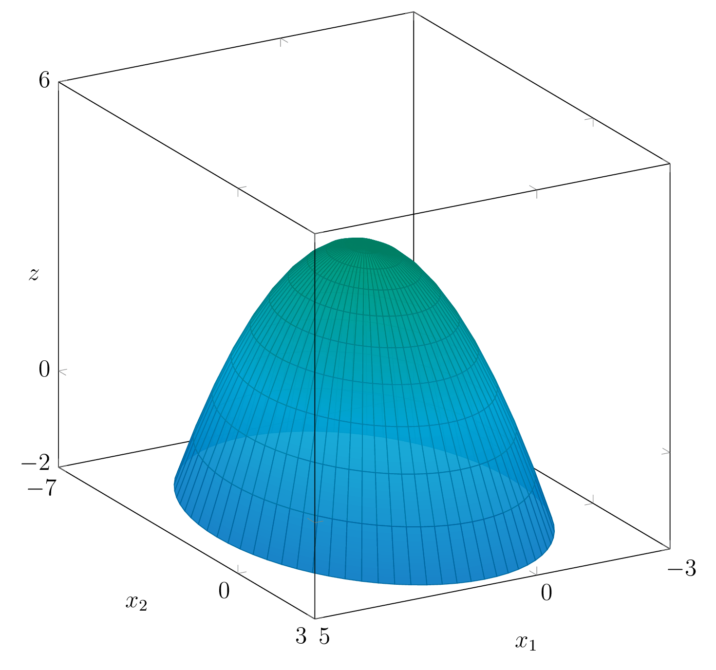
Fig. 8.2.3 The surface \(z = -\frac12x_1^2 - \frac14x_2^2 + x_1 - x_2 + 2\).

The shape of the surfaces is in most cases determined by the quadratic part \(\vect{x}^TA\vect{x}\). The linear part is then only relevant for the position.

Example 8.2.3

Consider the quadratic surface described by

\[ z = x_1^2 + 2x_1x_2 + 3 x_2^2. \]

We will apply the shift

\[ \tilde{x}_1 = x_1-3, \,\, \tilde{x}_2 = x_2 + 2, \]

so

\[ x_1 = \tilde{x}_1+3, \,\,x_2 = \tilde{x}_2- 2. \]

In the new variables \((\tilde{x}_1,\tilde{x}_2)\) we get

\[\begin{split} \begin{array}[t]{rcl} z &=&(\tilde{x}_1+3)^2 + 2(\tilde{x}_1+3)(\tilde{x}_2- 2) + 3 (\tilde{x}_2- 2)^2 \\ &=& \tilde{x}_1^2 + 2\tilde{x}_1\tilde{x}_2 + 3 \tilde{x}_2^2 +2\tilde{x}_1-6\tilde{x}_2 + 9. \end{array} \end{split}\]

Note that the quadratic parts are the same,

\[ x_1^2 + 2x_1x_2 - 3 x_2^2 \quad \text{versus} \quad \tilde{x}_1^2 + 2\tilde{x}_1\tilde{x}_2 - 3 \tilde{x}_2^2. \]

Example 8.2.4

The surfaces defined by

\[ \mathcal{S}_1: z = 2x_1^2 - 2x_1x_2 + x_2^2 \quad \text{and} \quad \mathcal{S}_2: z = 2x_1^2 - 2x_1x_2 + x_2^2 + 8x - 6y + 4 \]

are shifted versions of the same surface. Namely,

\[ 2x_1^2 - 2x_1x_2 + x_2^2 + 8x - 6y + 4 = 2(x_1+1)^2 - 2(x_1+1)(x_2-2) + (x_2-2)^2 - 6. \]

Thus \(\mathcal{S}_2\) is also described by

\[ z + 6 = 2(x_1+1)^2 - 2(x_1+1)(x_2-2) + (x_2-2)^2. \]

This means that if \(\mathcal{S}_1\) is translated over the vector \(\left(\begin{array}{c} -1 \\ 2 \\ -6 \end{array}\right)\) it becomes the surface \(\mathcal{S}_2\).

For the rest of the section we will therefore only look at the quadratic part \(\vect{x}^TA\vect{x}\).

One of the simplest quadratic forms results when we take \(A = I = I_n\), the identity matrix. Then we have

\[ q(\vect{x}) = \vect{x}^TI_n\vect{x} = \vect{x}^T\vect{x} =x_1^2 + x_2^2 + \cdots + x_n^2 = \vect{x}\ip\vect{x}. \]

For this quadratic form, it is clear that it will only take on non-negative values. And that

\[ q(\vect{x}) = 0 \quad \iff \quad \vect{x}=\vect{0}. \]

Such a quadratic form is called positive definite. In the next subsection we will learn how to find out whether an arbitrary quadratic form has this property.

8.2.2. Diagonalisation of quadratic forms

Let us first consider an example, to get some feeling for what is going on.

Example 8.2.5

Consider the quadratic form

\[\begin{split} q(x_1,x_2) = x_1^2 + 4x_1x_2 + 3x_2^2 = \begin{pmatrix}x_1 & x_2 \end{pmatrix} \begin{pmatrix}1 & 2 \\ 2 & 3 \end{pmatrix}\begin{pmatrix}x_1 \\ x_2 \end{pmatrix} = \vect{x}^TA\vect{x} . \end{split}\]

At first sight you might think that this quadratic form only takes on non-negative values. One way to show that this is not actually true is by completing squares.

\[ x_1^2 + 4x_1x_2 + 3x_2^2 = (x_1 + 2x_2)^2 - 4x_2^2 + 3x_2^2 = (x_1 + 2x_2)^2 - x_2^2. \]

For the last expression, that does not contain a cross term, we can see how we can get a negative outcome. We can make the first term equal to \(0\) by taking \(x_2 = 1\) and \(x_1 = -2\), and then have

\[ q(x_1,x_2) = q(-2,1) = (-2+2\cdot1)^2 - 1^2 = -1 < 0. \]

One way to describe in a more abstract/general way what we did in Example 8.2.5 is the following. We can introduce new variables \(y_1, y_2\) via the substitution

\[\begin{split} \left\{ \begin{array}{rr} y_1 =& x_1 + 2x_2 \\ y_2 =& x_2. \end{array} \right. \end{split}\]

For short,

\[\begin{split} \vect{y} = \left(\begin{array}{c} y_1 \\ y_2 \end{array}\right) = \left(\begin{array}{cc} 1 & 2 \\ 0 & 1 \end{array}\right)\left(\begin{array}{c} x_1 \\ x_2 \end{array}\right) = M\vect{x}. \end{split}\]

Then in terms of the new variables the quadratic form becomes

\[\begin{split} q(\vect{x}) = (x_1 + 2x_2)^2 - x_2^2 = y_1^2 - y_2^2 = \begin{pmatrix}y_1 & y_2 \end{pmatrix} \begin{pmatrix}1 & 0 \\ 0 &-1 \end{pmatrix}\begin{pmatrix}y_1 \\ y_2 \end{pmatrix} = \vect{y}^TD\vect{y}. \end{split}\]

Actually, it proves slightly advantageous to express the substitution as \(\vect{x} = P\vect{y}\) for an invertible matrix \(P\). We then have the following proposition.

quadratic form under a substitution

Proposition 8.2.2 (Quadratic form under a substitution)

The substitution \(\vect{x} = P\vect{y}\) brings the quadratic form

\[ q(\vect{x}) = \vect{x}^TA\vect{x} \]

over to

\[ \tilde{q}(\vect{y}) = \vect{y}^TP^TAP\vect{y}. \]

Proof of Proposition 8.2.2

If we put \(\vect{x} = P\vect{y}\) we get

\[ q(\vect{x}) = \vect{x}^TA\vect{x} = (P\vect{y})^TA(P\vect{y}) = \vect{y}^TP^T A P \vect{y}. \]

So in terms of \(\vect{y}\) we have the quadratic form

\[ \tilde{q}(\vect{y}) = \vect{y}^T \tilde{A} \vect{y} \]

where

\[ \tilde{A} = P^T A P. \]

Example 8.2.6

In Example 8.2.5 we considered the substitution

\[\begin{split} \vect{y} = \left(\begin{array}{cc} 1 & 2 \\ 0 & 1 \end{array}\right)\vect{x} \end{split}\]

or, equivalently

\[\begin{split} \vect{x} = \left(\begin{array}{cc} 1 & 2 \\ 0 & 1 \end{array}\right)^{-1}\vect{y} = \left(\begin{array}{cc} 1 & -2 \\ 0 & 1 \end{array}\right)\vect{y} = P \vect{y} \end{split}\]

to the quadratic form

\[\begin{split} q(\vect{x}) = \vect{x}^T\left(\begin{array}{cc} 1 & 2 \\ 2 & 3 \end{array}\right)\vect{x}. \end{split}\]

We then have

\[\begin{split} \begin{array}{rcl} P^TAP &=& \begin{pmatrix} 1 & -2 \\ 0 & 1 \end{pmatrix}^T\begin{pmatrix} 1 & 2 \\ 2 & 3 \end{pmatrix}\begin{pmatrix} 1 & -2 \\ 0 & 1 \end{pmatrix} \\ &=& \begin{pmatrix} 1 & 0 \\ -2 & 1 \end{pmatrix}\begin{pmatrix} 1 & 0 \\ 2 & -1 \end{pmatrix} = \begin{pmatrix} 1 & 0 \\ 0 & -1 \end{pmatrix}. \end{array} \end{split}\]

According to Proposition 8.2.2 we then get the quadratic form

\[\begin{split} \tilde{q}(y) = \vect{y}^TP^TAP\vect{y} = \vect{y}^T\left(\begin{array}{cc} 1 & 0 \\ 0 & -1 \end{array}\right)\vect{y} = y_1^2 - y_2^2. \end{split}\]

This agrees with what we derived in Example 8.2.5.

The technique of completing the squares is one way to ‘diagonalise’ a quadratic form. It may be turned into an algorithm that also works for quadratic forms in \(n\) variables, but we will not pursue that track. There is a route that is more in line with the properties of symmetric matrices.

Suppose \(A\) is a symmetric matrix. We have seen (cf. Theorem 8.1.1) that it can be written as

\[ A = QDQ^{-1} \]

for an orthogonal matrix \(Q\). The diagonal matrix \(D\) has the eigenvalues of \(A\) on its diagonal.

Since \(Q\) is an orthogonal matrix, we have

\[ A = QDQ^{-1} = QDQ^T. \]

If we compare this to Proposition 8.2.2 the following proposition results.

Proposition 8.2.3

Suppose \(q(\vect{x})\) is a quadratic form with matrix \(A\), i.e.,

\[ q(\vect{x}) = \vect{x}^TA\vect{x}. \]

Let \(Q\) be an orthogonal matrix diagonalising \(A\). That is, \(A = QDQ^{-1}\).

Applying the substitution \(\vect{x} = Q\vect{y}\) then yields the quadratic form

\[ \vect{y}^TD\vect{y} = \lambda_1y_1^2 + \lambda_2y_2^2 + \cdots + \lambda_ny_n^2, \]

where \(\lambda_1, \ldots, \lambda_n\) are the eigenvalues of the matrix \(A\).

Proof of Proposition 8.2.3

If we make the substitution \(\vect{x} = Q\vect{y}\) we find that

\[ \vect{x}^TA\vect{x} = (Q\vect{y})^TQDQ^{-1}(Q\vect{y}) = \vect{y}^TQ^TQD Q^{-1}Q\vect{y} = \vect{y}^TD\vect{y}. \]

The last expression is indeed of the form

\[\begin{split} \vect{y}^T\begin{pmatrix} \lambda_1 & 0 & \cdots & 0 \\ 0 & \lambda_2 & \cdots & 0 \\ \vdots & \vdots & \ddots & \vdots \\ 0 & 0 & \cdots & 0 \end{pmatrix}\vect{y} = \lambda_1y_1^2 + \lambda_2y_2^2 + \cdots + \lambda_ny_n^2, \end{split}\]

where \(\lambda_1,\lambda_2, \ldots, \lambda_n\) are the eigenvalues of \(A\).

Let us see how the construction of Proposition 8.2.3 works out in an earlier example.

Example 8.2.7

Consider again the matrix \(A = \left(\begin{array}{cc} 1 & 2 \\ 2 & 3 \end{array}\right)\) of Example 8.2.6.

Its characteristic polynomial is given by

\[ p_A(\lambda) = (1-\lambda)(3-\lambda)-4 = \lambda^2 - 4\lambda - 1. \]

The eigenvalues are

\[ \lambda_1 = 2 + \sqrt{5}, \quad \lambda_2 = 2 - \sqrt{5}. \]

So if we take \(Q = \begin{pmatrix} \vect{q}_1 & \vect{q}_2 \end{pmatrix}\), where \(\vect{q}_1\) and \(\vect{q}_2\) are corresponding eigenvectors of unit length, we find that the substitution \(\vect{x} = Q\vect{y}\) leads to

\[ \vect{x}^TA\vect{x} \,\stackrel{\scriptsize \vect{x} = Q\vect{y}}{\longrightarrow}\, \vect{y}^TD\vect{y} = (2 + \sqrt{5})y_1^2 - (2 - \sqrt{5})y_2^2. \]

Since \((2 + \sqrt{5})> 0\) and \((2 - \sqrt{5})<2-2=0\) we may again conclude that the quadratic form takes on both positive and negative values.

Remark 8.2.1

In Example 8.2.6 and Example 8.2.7 we applied two different substitutions to the same quadratic form with the matrix \(A = \left(\begin{array}{cc} 1 & 2 \\ 2 & 3 \end{array}\right)\).

They led to the two different quadratic forms

\[\begin{split} \vect{y}^TD_1\vect{y} = \vect{y}^T\begin{pmatrix}1 & 0\\ 0 & -1 \end{pmatrix}\vect{y} \quad \text{and} \quad \vect{y}^TD_2\vect{y} = \vect{y}^T\begin{pmatrix}2 + \sqrt{5} & 0\\ 0 & 2 - \sqrt{5}\end{pmatrix}\vect{y}. \end{split}\]

The diagonal matrices do not seem to have much in common. However, they do.

It can be shown that if for a symmetric \(n\times n\)-matrix \(A\) it holds that

\[ P_1^TAP_1 = D_1 \quad \text{and} \quad P_2^TAP_2 = D_2, \]

for two invertible matrices \(P_1\), \(P_2\), then the signs of the values on the diagonals of \(D_1\) and \(D_2\) match in the following sense:

if \(p_1\), \(p_2\) denote the numbers of positive diagonal elements of \(D_1, D_2\), and \(n_i\) are the numbers of negative diagonal elements, then

\[ p_1 = p_2 \quad \text{and} \quad n_1 = n_2. \]

It follows that the numbers of zeros on the diagonals, \(n - p_i - n_i\), \(i = 1,2\), must also be equal for the two matrices.

In the two examples we see that \(p_1 = p_2 = 1\) and also \(n_1 = n_2 = 1\), in accordance with the statement.

The property is known as Sylvester’s Law of Inertia.

Grasple Exercise 8.2.1

To garner some evidence for Sylvester’s Law of Inertia.

Click to show/hide

The following proposition is a direct consequence of the diagonalisation (Proposition 8.2.3).

Proposition 8.2.4

Let \(q(x) = \vect{x}^TA\vect{x}\) be the quadratic form with matrix \(A\) and suppose that \(A\) has the (ordered) eigenvalues \(\lambda_1 \geq \lambda_2 \geq \cdots \geq \lambda_n\). Then the maximum and the minimum value attained by \(q(\vect{x})\) under the constraint \(\norm{\vect{x}} = 1\) are \(\lambda_1\) and \(\lambda_n\).

The proof contains the same type of reasoning as the proof of Proposition 8.1.4.

Proof of Proposition 8.2.4

Suppose that \(\vect{u}_1, \vect{u}_2,\ldots,\vect{u}_n\) is an orthonormal basis of eigenvectors for \(A\) for the eigenvalues \(\lambda_1 \geq \cdots \geq \lambda_n\).

First of all

\[ q(\vect{u}_1) = \vect{u}_1^TA\vect{u}_1 = \vect{u}_1^T(A\vect{u}_1) = \vect{u}_1^T(\lambda_1\vect{u}_1) = \lambda_1\vect{u}_1^T\vect{u}_1 = \lambda_1. \]

Likewise \(q(\vect{u}_n) = \lambda_n\), so \(q(\vect{x})\) does take on the values \(\lambda_1\) and \(\lambda_n\).

Next, for an arbitrary unit vector \(\vect{x}\), which can always be written as

\[ c_1\vect{u}_1 + c_2\vect{u}_2 + \cdots + c_n\vect{u}_n, \quad \text{with} \quad c_1^2 + c_2^2 + \cdots + c_n^2 = 1 \]

(cf. proof of Proposition 8.1.4), we deduce that

\[\begin{split} \begin{array}{rcl} \vect{x}^TA\vect{x} &=& (c_1\vect{u}_1 + \cdots + c_n\vect{u}_n)^T(c_1\lambda_1\vect{u}_1 + \cdots + c_n\lambda_n\vect{u}_n) \\ &=& c_1^2\lambda_1\vect{u}_1^T\vect{u}_1 + \cdots + c_n^2\lambda_n\vect{u}_n^T\vect{u}_n \\ &=& c_1^2\lambda_1 + \cdots + c_n^2\lambda_n. \end{array} \end{split}\]

All cross terms \(\vect{u}_i^T\vect{u}_j\) with \(i\neq j\) drop out since \(\vect{u}_i\ip\vect{u}_j=0\), for \(i\neq j\), and \(\vect{u}_i^T\vect{u}_i = 1\) by the assumption that the vectors \(\mathbf{u}_i\) are unit vectors.

Now, invoking \(\lambda_1 \geq \lambda_2 \geq \cdots \geq \lambda_n\) and \(c_1^2 + c_2^2 + \cdots +c_n^2 = 1\), we see that

\[\begin{split} \begin{array}{rcl} \lambda_n = \left(c_1^2 +c_2^2 +\cdots + c_n^2\right)\lambda_n &=& c_1^2\lambda_n +c_2^2\lambda_n +\cdots + c_n^2\lambda_n \\ &\leq& c_1^2\lambda_1 +c_2^2\lambda_2 +\cdots + c_n^2\lambda_n, \end{array} \end{split}\]

and also

\[ \lambda_1 \geq c_1^2\lambda_1 +c_2^2\lambda_2 +\cdots + c_n^2\lambda_n, \]

so we may conclude that indeed

\[ \lambda_n \,\leq\, c_1^2\lambda_1 +c_2^2\lambda_2 +\cdots + c_n^2\lambda_n \,\leq\, \lambda_1, \]

where the expression in the middle is equal to our \(\vect{x}^T A \vect{x} = q(\vect{x})\).

8.2.3. Positive definite matrices

Let’s start with a list of definitions.

negative semi-definiteclassification of quadratic formsindefinite quadratic formpositive definite matrixpositive semi-definitenegative definitepositive definite quadratic form

Definition 8.2.1 (Classification of Quadratic Forms)

Let \(A\) be a symmetric matrix and \(q_A(\vect{x}) = \vect{x}^TA\vect{x}\) the corresponding quadratic form.

• \(q_A\) is called a positive definite quadratic form if \(q_A(\vect{x}) > 0\) for all \(\vect{x} \neq \vect{0}\).

• \(q_A\) is called positive semi-definite if \(q_A(\vect{x}) \geq 0\) for all \(\vect{x} \).

• \(q_A\) is called negative definite if \(q_A(\vect{x}) < 0\) for all \(\vect{x} \neq \vect{0}\).

• \(q_A\) is called negative semi-definite if \(q_A(\vect{x}) \leq 0\) for all \(\vect{x} \).

If none of the above applies, then \(q_A\) is called an indefinite quadratic form.

The same classification is used for symmetric matrices. E.g., \(A\) is a positive definite matrix if the corresponding quadratic form is positive definite.

Note that every quadratic form \(\vect{x}^TA\vect{x}\) gets the value \(0\) when \(\vect{x}\) is the zero vector. That is the reason we exclude the zero vector in the definition of positive/negative definite.

The classification of a quadratic form follows immediately from the eigenvalues of its matrix.

Theorem 8.2.1

Suppose \(q_A(\vect{x}) = \vect{x}^TA\vect{x}\) for the symmetric \(n \times n\)-matrix \(A\). Let \(\lambda_1, \ldots, \lambda_n\) be the complete set of (real) eigenvalues of \(A\)

Then

• \(q_A\) is positive definite if and only if all eigenvalues are positive.

• \(q_A\) is positive semi-definite if and only if all eigenvalues are non-negative.

• \(q_A\) is negative definite if and only if all eigenvalues are negative.

• \(q_A\) is negative semi-definite if and only if all eigenvalues are non-positive.

And lastly

• \(q_A\) is indefinite if at least one eigenvalue is positive and at least one eigenvalue is negative.

Proof of Theorem 8.2.1

This immediately follows from Proposition 8.2.3. If we make the substitution \(\vect{x} = Q\vect{y}\) with the matrix \(Q\) of the orthogonal diagonalisation, i.e.,

\[\begin{split} A = QDQ^{-1} = QDQ^T, \quad D = \left(\begin{array}{cccc} \lambda_1 & 0 & \cdots & 0 \\ 0 & \lambda_2 & \cdots & 0 \\ \vdots & \vdots & \ddots &\vdots\\ 0 & 0 & \cdots & \lambda_n \end{array}\right), \end{split}\]

the quadratic form transforms to

\[ \tilde{q}(\vect{y}) = \vect{y}^TD\vect{y} = \lambda_1y_1^2 + \cdots + \lambda_ny_n^2. \]

Let us consider the case where all eigenvalues \(\lambda_i\) are positive. Then the expression for \(\tilde{q}(\vect{y})\) is positive for all \(\vect{y} \neq \vect{0}\). It remains to show that then also \(q(\vect{x}) > 0\) for all vectors \(\vect{x}\neq \vect{0}\).

Since \(Q\) is an orthogonal matrix it is also an invertible matrix. So any non-zero vector \(\vect{x}\) can be written as

\[ \vect{x} = Q\vect{y} \]

for a (unique) non-zero vector \(\vect{y}\).

As a consequence, for any non-zero vector \(\vect{x}\) we have

\[ \vect{x}^TA\vect{x} = (Q\vect{y})^TA(Q\vect{y}) = \vect{y}^TQ^TAQ\vect{y} = \vect{y}^TD\vect{y} > 0. \]

Likewise the other possibilities of the signs of the eigenvalues may be checked.

Exercise 8.2.1

Verify the validity of the second statement made in Theorem 8.2.1.

Solution to Exercise 8.2.1

The transformed quadratic form is still

\[ \tilde{q}(\vect{y}) = \vect{y}^TD\vect{y} = \lambda_1y_1^2 + \cdots + \lambda_ny_n^2, \]

and \(q_A(\vect{x})=\tilde{q}(\vect{y})\) with \(\vect{x} = Q\vect{y}\).

Now we can chain the following equivalent statements:

\[\begin{split} \begin{align*} \text{$q_A$ is positive definite} &\iff \text{$q_A(\vect{x})\geq0$ for all $\vect{x}$} \\ &\iff \text{$\tilde{q}(\vect{y})\geq0$ for all $\vect{y}$} \\ &\iff \text{$\lambda_1y_1^2 + \cdots + \lambda_ny_n^2\geq0$ for all $\vect{y}$} \\ &\iff \text{$\lambda_j\geq0$ for $j=1,\ldots,n$}. \end{align*} \end{split}\]

Example 8.2.8

Consider the quadratic form

\[ q(x_1,x_2,x_3) = 2x_1^2 + x_2^2 +x_3^2 - 2x_1x_2 - 2x_1x_3. \]

The matrix of this quadratic form is

\[\begin{split} A = \left(\begin{array}{cc} 2 & -1 & -1 \\ -1 & 1 & 0 \\ -1 & 0 & 1 \end{array}\right). \end{split}\]

The eigenvalues of \(A\) are computed as

\[ \lambda_1 = 3, \quad \lambda_2 = 1, \quad \lambda_3 = 0. \]

With Theorem 8.2.1 in mind, we can conclude that the quadratic form is positive semi-definite but not positive definite.

Exercise 8.2.2

This exercise nicely recapitulates the ideas of the section. There is a cameo of the concept of completing the square, but that is of minor importance.

1. Show that the quadratic from in Example 8.2.8 can be rewritten as follows

   (8.2.2)\[q(x_1,x_2,x_3) = 2(x_1 - \tfrac12x_2 - \tfrac12x_3)^2 + \tfrac12(x_2 - x_3)^2.\]

2. What is the corresponding transformation \(\vect{y} = P\vect{x}\) that brings the quadratic form in diagonal form \(\vect{y}^TD_2\vect{y}\), and what is the diagonal matrix \(D_2\)?

3. By inspection of \(D_2\) find the classification of \(q\).

4. By inspection of Equation (8.2.2), find a non-zero vector \(\vect{x}\) for which \(q(\vect{x}) = 0\).

5. Check that the vector you found in iii. is an eigenvector of the matrix of the quadratic form, i.e., \(A = \left(\begin{array}{cc} 2 & -1 & -1 \\ -1 & 1 & 0 \\ -1 & 0 & 1 \end{array}\right)\).

Solution to Exercise 8.2.2

1. We perform direct computations:

   \[\begin{split} \begin{align*} q(x_1,x_2,x_3) &= 2x_1^2 + x_2^2 +x_3^2 - 2x_1x_2 - 2x_1x_3 \\ &= 2\left(x_1^2 - x_1x_2 - x_1x_3\right)+ x_2^2 +x_3^2 \\ &= 2\left(\left(x_1 - \frac12x_2 - \frac12x_3\right)^2-\left(\frac12x_2+\frac12x_3\right)^2\right)+ x_2^2 +x_3^2 \\ &= 2\left(\left(x_1 - \frac12x_2 - \frac12x_3\right)^2-\frac14x_2^2-\frac14x_2x_3-\frac14x_3^2\right)+ x_2^2 +x_3^2 \\ &= 2\left(x_1 - \frac12x_2 - \frac12x_3\right)^2-\frac12x_2^2-\frac12x_2x_3-\frac12x_3^2+ x_2^2 +x_3^2 \\ &= 2\left(x_1 - \frac12x_2 - \frac12x_3\right)^2+\frac12x_2^2-\frac12x_2x_3+\frac12x_3^2 \\ &= 2\left(x_1 - \frac12x_2 - \frac12x_3\right)^2+\frac12\left(x_2^2-x_2x_3+x_3^2\right) \\ &= 2(x_1 - \tfrac12x_2 - \tfrac12x_3)^2 + \tfrac12(x_2 - x_3)^2. \end{align*} \end{split}\]

2. We only present the answer here:

   \[\begin{split} P=\begin{pmatrix} -\frac{2}{\sqrt6} & 0 & \frac{1}{\sqrt2} \\ \frac{1}{\sqrt6} & -\frac{1}{\sqrt2} & \frac{1}{\sqrt2} \\ \frac{1}{\sqrt6}& \frac{1}{\sqrt2} & \frac{1}{\sqrt2} \end{pmatrix}\text{ and }D_2=\begin{pmatrix}3&0&0\\0&1&0\\0&0&0\end{pmatrix} \end{split}\]

3. \(q\) is positive semi-definite.

4. The last term of Equation (8.2.2) gives rise to chosing \(x_2=x_3\). The first term then indicates \(x_1=\frac12x_2+\frac12x_3=x_3\). Chosing \(x_3=1\) gives \(x_2=1\) and \(x_1=1\). In vector form:

   \[\begin{split} \vect{x}=\begin{pmatrix}1\\1\\1\end{pmatrix}. \end{split}\]

5. The vector \(\vect{x}=\begin{pmatrix}1\\1\\1\end{pmatrix}\) is a non-zero scalar multiple of the third column of \(P\), so it is an eigenvector.

8.2.4. Conic sections

A conic section or conic is a curve that results when a circular cone is intersected with a plane.
Figure 8.2.4 shows the different shapes when the plane is not going through the apex.

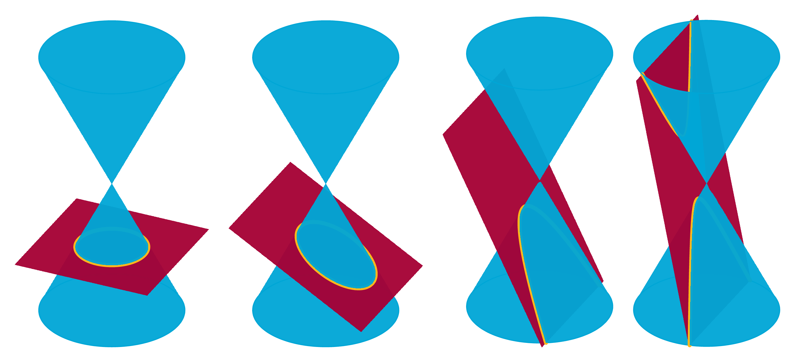
Fig. 8.2.4 Intersections of a cone with several planes (not going through the apex).

The resulting curve is then either a hyperbola, a parabola or an ellipse, with as special ellipse the circle. If the plane does go through the apex of the cone the conic section is called degenerate.

Exercise 8.2.3

Describe the (three) possible degenerate forms of conic sections. That is, what are the three different forms that result when a cone is intersected with a plane that goes through the apex?

Solution to Exercise 8.2.3

There are three essentially different situations.

A plane through the apex may have the apex as unique common point with the cone. Then the conic (inter)section is just this one point.

If (as in the central image in Figure 8.2.5) the plane is close to vertical, it will intersect the cone in two lines through the apex.

The transition between these situations is when the plane is tangent to the cone. This yields the last possible conic section, a line.

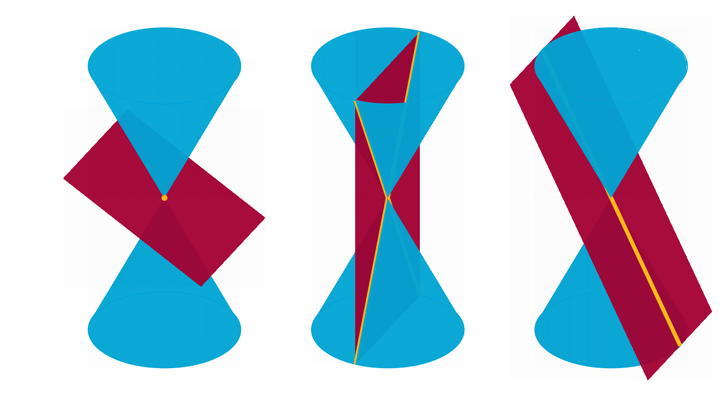
Fig. 8.2.5 The three degenerate conic sections.

In the plane all non-degenerate conic sections may be described by a quadratic equation

(8.2.3)\[ax_1^2 + b x_1x_2 + cx_2^2 + dx_1 + ex_2 + f = 0,\]

where both the parameter \(f\) and at least one of the parameters \(a,b,c\) are not equal to zero.

Example 8.2.9

The curve given by the equation \(x_1^2 + x_2^2 - 25 = 0\) is a circle with radius \(5\).

The equation \(x_1^2 - x_2 - 2x_1 + 5 = 0\) gives a parabola with vertex (‘top’) at \((1, 4)\) and the line \(x_1 = 1\) as axis of symmetry.

If the parameters \(d\) and \(e\) in Equation (8.2.3) are zero, the equation

(8.2.4)\[ax_1^2 + bx_1x_2 + cx_2^2 + f = 0\]

is said to represent a central conic. When \(b = 0\) as well,

(8.2.5)\[ax_1^2 + cx_2^2 + f = 0\]

defines a central conic in standard position. Such a conic is symmetric with respect to both coordinate axes.

If all parameters \(a,c,f\) in Equation (8.2.5) are non-zero the equation can be rewritten in one of the two standard forms

(8.2.6)\[(I) \,\, \dfrac{x_1^2}{r_1^2} + \dfrac{x_2^2}{r_2^2} = 1, \quad\quad (II) \,\, \dfrac{x_1^2}{r_1^2} - \dfrac{x_2^2}{r_2^2} = \pm 1,\]

where we may assume that \( r_1,r_2 > 0\).

In case \((I)\) the equation describes an ellipse if \(r_1 \neq r_2\) and a circle if \(r_1 = r_2\).

In case \((II)\) the resulting curve is a hyperbola, with the lines \(x_2 = \pm\dfrac{r_2}{r_1}x_1\) as asymptotes.

Both curves have the coordinates axes as axes of symmetry. In this context they are also called the principal axes. See Figure 8.2.6.

Fig. 8.2.6 (Standard) Hyperbola and Ellipse.

Example 8.2.10

The equation

\[ 4x_1^2 + 9x_2^2 - 25 = 0 \]

can be rewritten as

\[ \dfrac{4x_1^2}{25} + \dfrac{9x_2^2}{25} = 1, \]

and a bit further to the standard form

\[ \dfrac{x_1^2}{(5/2)^2} + \dfrac{x_2^2}{(5/3)^2} = 1. \]

The corresponding curve is an ellipse with the coordinate axes as principal axes and with \(-5/2 \leq x_1 \leq 5/2\) and \(-5/3 \leq x_2 \leq 5/3\).

Likewise

\[ 4x_1^2 - x_2^2 + 9 = 0 \quad \iff \quad \dfrac{x_1^2}{(3/2)^2} - \dfrac{x_2^2}{3^2} = -1. \]

When rewritten in the form

\[ x_2 = \pm \sqrt{9 + 4x_1^2} = \pm2x_1\sqrt{\dfrac{9}{4x_1^2} + 1} \]

it is seen that the lines \(x_2 = \pm 2x_1\) are asymptotes. Namely, if \(x_1 \to \pm \infty\), then

\[ \sqrt{\dfrac{9}{4x_1^2} + 1} \,\to\, \sqrt{0+1} = 1. \]

If in Equation (8.2.4) the parameter \(b\) is not equal to zero, the principal axes can be found by diagonalisation of the quadratic form

\[\begin{split} ax_1^2 + 2bx_1x_2 + cx_2^2 = \begin{pmatrix} x_1 & x_2 \end{pmatrix}\begin{pmatrix} a & b \\ b & c\end{pmatrix}\begin{pmatrix} x_1 \\ x_2 \end{pmatrix}. \end{split}\]

The next proposition explains how.
For notational convenience we have denoted the coefficient of the cross term as \(2b\).

Proposition 8.2.5

Suppose the conic \(\mathcal{C}\) is defined by the equation

\[ ax_1^2 + 2bx_1x_2 + cx_2^2 = k, \]

where \(a,b,c\) are not all equal to zero, and \(k \neq 0\).

Then the principal axes are the lines generated by the eigenvectors of the matrix

\[\begin{split} A = \begin{pmatrix} a & b \\ b & c \end{pmatrix}. \end{split}\]

We will not give a proof of Proposition 8.2.5, but instead we will give two illustrative examples.

Example 8.2.11

We consider the quadratic form

(8.2.7)\[x_1^2 - 4x_1x_2 + x_2^2 = 4.\]

Since

\[\begin{split} x_1^2 - 4x_1x_2 + x_2^2 = \begin{pmatrix} x_1 & x_2 \end{pmatrix}\begin{pmatrix} 1 & -2 \\ -2 & 1\end{pmatrix}\begin{pmatrix} x_1 \\ x_2 \end{pmatrix}, \end{split}\]

Proposition 8.2.5 tells us we have to look for eigenvectors of the matrix

\[\begin{split} A = \begin{pmatrix} 1 & -2 \\ -2 & 1\end{pmatrix}. \end{split}\]

The usual computations yield the following eigenvalues and eigenvectors:

\[\begin{split} \lambda_1 = 3,\,\vect{v}_1 = \begin{pmatrix} 1 \\ -1\end{pmatrix},\quad \lambda_2 = -1,\,\vect{v}_2 = \begin{pmatrix} 1 \\ 1\end{pmatrix}. \end{split}\]

The eigenvectors are orthogonal, as they should, for a symmetric matrix. We see that \(A\) can be orthogonally diagonalised as

\[\begin{split} A = QDQ^{-1} = QDQ^T, \quad Q = \frac{1}{\sqrt{2}}\begin{pmatrix} 1 & 1 \\ -1 & 1\end{pmatrix}, \,\, D = \begin{pmatrix} 3 & 0 \\ 0 & -1\end{pmatrix}. \end{split}\]

The substitution \(\vect{x} = Q\vect{y}\) yields

\[ \vect{x}^T A \vect{x} = \vect{y}^T Q^TAQ \vect{y} = \vect{y}^T D \vect{y} = 3y_1^2 - y_2^2. \]

So in the coordinates \(y_1\) and \(y_2\) the equation becomes

\[ 3y_1^2 - y_2^2 = 4. \]

From this we can already conclude that the curve defined by Equation (8.2.7) is a hyperbola. The principal axes in the \(x_1\)-\(x_2\)-plane are the lines given by

\[\begin{split} \mathcal{L}_1: \begin{pmatrix} x_1 \\ x_2\end{pmatrix} = c \begin{pmatrix} 1 \\ -1\end{pmatrix} \quad \text{and} \quad \mathcal{L}_2: \begin{pmatrix} x_1 \\ x_2\end{pmatrix} = c \begin{pmatrix} 1 \\ 1\end{pmatrix} \end{split}\]

The asymptotes in the coordinates \(y_1, y_2\) are the lines

\[\begin{split} y_2 = \pm\sqrt{3} y_1, \,\, \text{or} \,\,\, \begin{pmatrix} y_1 \\ y_2\end{pmatrix} = c \begin{pmatrix} 1 \\ \pm \sqrt{3}\end{pmatrix}. \end{split}\]

Since

\[\begin{split} \begin{pmatrix} x_1 \\ x_2\end{pmatrix} = \dfrac{1}{\sqrt{2}} \begin{pmatrix} 1 & 1 \\ -1 & 1\end{pmatrix}\begin{pmatrix} y_1 \\ y_2\end{pmatrix} = \begin{pmatrix} \cos\left(-\frac14\pi\right) & -\sin\left(-\frac14\pi\right) \\ \sin\left(-\frac14\pi\right) & \cos\left(-\frac14\pi\right)\end{pmatrix}\begin{pmatrix} y_1 \\ y_2\end{pmatrix} \end{split}\]

we find the asymptotes in the \(x_1\)-\(x_2\)-plane by rotating the lines \(y_2 = \pm\sqrt{3}y_1\) over an angle \(-\frac14\pi\). This leads to the direction vectors of the asymptotes in the \(x_1\)-\(x_2\)-plane as

\[\begin{split} \dfrac{1}{\sqrt{2}} \begin{pmatrix} 1 & 1 \\ -1 & 1\end{pmatrix}\begin{pmatrix} 1 \\ 3\end{pmatrix} = \dfrac{1}{\sqrt{2}} \begin{pmatrix} 4 \\ 2\end{pmatrix},\,\, \,\, \dfrac{1}{\sqrt{2}} \begin{pmatrix} 1 & 1 \\ -1 & 1\end{pmatrix}\begin{pmatrix} 1 \\ -3\end{pmatrix} = \dfrac{1}{\sqrt{2}} \begin{pmatrix} -2 \\ -4\end{pmatrix}. \end{split}\]

They can be simplified to the direction vectors \( \begin{pmatrix} 2 \\ 1\end{pmatrix}\) and \(\begin{pmatrix} 1 \\ 2\end{pmatrix}\).

Example 8.2.12

We consider the quadratic form

(8.2.8)\[3x_1^2 + 4x_1x_2 + 6x_2^2 = 36.\]

Here we have

\[\begin{split} 3x_1^2 + 4x_1x_2 + 6x_2^2 = \begin{pmatrix} x_1 & x_2 \end{pmatrix}\begin{pmatrix} 3 & 2 \\ 2 & 6\end{pmatrix}\begin{pmatrix} x_1 \\ x_2 \end{pmatrix}, \end{split}\]

so now we have to look for eigenvalues and eigenvectors of the matrix

\[\begin{split} A = \begin{pmatrix} 3 & 2 \\ 2 & 6\end{pmatrix}. \end{split}\]

They are found to be

\[\begin{split} \lambda_1 = 2,\,\vect{v}_1 = \begin{pmatrix} 2 \\ -1\end{pmatrix},\quad \lambda_2 = 7,\,\vect{v}_2 = \begin{pmatrix} 1 \\ 2\end{pmatrix}. \end{split}\]

We orthogonally diagonalise \(A\) as

\[\begin{split} A = QDQ^{-1} = QDQ^T, \quad Q = \frac{1}{\sqrt{5}}\begin{pmatrix} 2 & 1 \\ -1 & 2\end{pmatrix}, \,\, D = \begin{pmatrix} 2 & 0 \\ 0 & 7\end{pmatrix}. \end{split}\]

The substitution \(\vect{x} = Q\vect{y}\) yields the quadratic form

\[ 2y_1^2 + 7y_2^2 = 36, \]

or

\[ \dfrac{y_1^2}{(3\sqrt{2})^2} + \dfrac{y_2^2}{(6/\sqrt{7})^2} = 1. \]

This is an ellipse in the \(y_1\)-\(y_2\)-plane with long axis \(6\sqrt{2}\), the length of the line segment from \((-3\sqrt{2},0)\) to \((3\sqrt{2},0)\), and short axis \(\dfrac{12}{\sqrt{7}}\).

For the ellipse in the \(x_1\)-\(x_2\)-plane we find the principal axes

\[\begin{split} \begin{pmatrix} x_1 \\ x_2\end{pmatrix} = c\vect{v}_1 = c\begin{pmatrix} 2 \\ -1\end{pmatrix} \quad \text{and}\quad \begin{pmatrix} x_1 \\ x_2\end{pmatrix} = c\vect{v}_2 = c\begin{pmatrix} 1 \\ 2\end{pmatrix}. \end{split}\]

See Figure Fig. 8.2.7

Fig. 8.2.7 The ellipse with its principal axes.

Exercise 8.2.4

What happens if in Equation (8.2.4) the coefficient \(f\) is equal to zero? (There are actually three cases to consider!)

Solution to Exercise 8.2.4

We have to look at the solutions \((x_1, x_2)\) of the equation \(ax_1^2 + bx_1x_2 + cx_2^2 = 0\), where not all three coefficients \(a,b,c\) are zero.

We can rewrite the equation as

\[\begin{split} \vect{x} ^TA\vect{x} = \vect{0},\text{ with }\vect{x}=\begin{pmatrix} x_1 & x_2 \end{pmatrix}\text{ and }A=\begin{pmatrix} a & b \\ b & c \end{pmatrix}. \end{split}\]

As \(A\) is symmetric, it can be orthogonally diagonalised as \(A=QDQ^T\), with \(D\) a diagonal matrix with the eigenvalues \(\lambda_1, \lambda_2\) of \(A\) on the diagonal and \(Q\) an orthogonal matrix with the corresponding eigenvectors as columns.

The substitution \(\vect{x} = Q\vect{y}\) transforms the equation to

\[ \vect{y}^TD\vect{y} = 0, \]

or equivalently

(8.2.9)\[\lambda_1y_1^2 + \lambda_2y_2^2 = 0.\]

We now consider three cases: \(\lambda_1\lambda_2 > 0\), \(\lambda_1\lambda_2 < 0\) and \(\lambda_1\lambda_2 = 0\).

For \(\lambda_1\lambda_2 > 0\), the only solution to (8.2.9) is \(\vect{y} = \vect{0}\), which means that the only solution to the original equation is \(\vect{x} = \vect{0}\), i.e. the conic section is the point \((x_1,x_2)=(0,0)\).

If \(\lambda_1\lambda_2 < 0\), the two solutions to (8.2.9) are

\[ y_2 = \pm \sqrt{-\frac{\lambda_1}{\lambda_2}}y_1, \]

which are are with respect to the \((y_1,y_2)\)-coordinates two intersecting lines through the origin, with slopes \(\pm \sqrt{-\frac{\lambda_1}{\lambda_2}}\). As the transformation \(\vect{x} = Q\vect{y}\) is invertible, the two intersecting lines in the \((y_1,y_2)\)-plane are transformed to two intersecting lines through the origin in the \((x_1,x_2)\)-plane.

Finally, consider the case \(\lambda_1\lambda_2 = 0\). Then one of the eigenvalues is zero, say \(\lambda_1 = 0\), and the other is non-zero, say \(\lambda_2 \neq 0\). The equation (8.2.9) then becomes

\[ \lambda_2y_2^2 = 0, \]

which has the solution \(y_2 = 0\). The other variable \(y_1\) can take any value, so the solution set is the line \(y_2 = 0\) in the \((y_1,y_2)\)-plane. The transformation \(\vect{x} = Q\vect{y}\) is still invertible, so the solution set in the \((x_1,x_2)\)-plane is also a line, namely the line through the origin with direction vector \(\vect{v}_1\), the eigenvector corresponding to the zero eigenvalue.

8.2.5. Grasple exercises

Grasple Exercise 8.2.2

To write down the matrix of a quadratic form in three variables.

Click to show/hide

Grasple Exercise 8.2.3

To write down the matrix of a quadratic form in three variables.

Click to show/hide

Grasple Exercise 8.2.4

To perform a change of variables for a quadratic form \(\vect{x}^TA\vect{x}\) in two variables.

Click to show/hide

Grasple Exercise 8.2.5

To classify a \(3\times3\)-matrix of which the characteristic polynomial is given.

Click to show/hide

Grasple Exercise 8.2.6

To classify a quadratic form in two variables.

Click to show/hide

Grasple Exercise 8.2.7

To classify a quadratic form in two variables.

Click to show/hide

Grasple Exercise 8.2.8

To classify two quadratic forms in two variables.

Click to show/hide

Grasple Exercise 8.2.9

For which value of a parameter \(\beta\) is a quadratic form in two variables indefinite?

Click to show/hide

Grasple Exercise 8.2.10

To describe three central conic sections geometrically.

Click to show/hide

Grasple Exercise 8.2.11

Natural sequel to previous exercise.

Click to show/hide

Grasple Exercise 8.2.12

For which parameter \(a\) is a conic section \(\vect{x}^TA\vect{x} =1\) an ellipse/hyperbola/something else?

Click to show/hide

Grasple Exercise 8.2.13

Maximising \(\vect{x}^TA\vect{x}\) under the restriction \(\norm{\vect{x}}=1\), for a \(2\times2\)-matrix \(A\).

Click to show/hide

The following exercises are a more theoretical.

Grasple Exercise 8.2.14

True or false? If \(A\) is a positive definite matrix, then the diagonal of \(A\) is positive (v.v.).

Click to show/hide

Grasple Exercise 8.2.15

If \(A\) and \(B\) are symmetric matrices with positive eigenvalues, what about \(A+B\)?

Click to show/hide

Grasple Exercise 8.2.16

Two True/False questions about vectors \(\vect{x}\) for which \(\vect{x}^TA\vect{x} = 0\).

Click to show/hide