Wigner functions of mixed states

Here, we will explore the Wigner quasiprobability distributions of “mixed states” (or, more accurately, of mixed ensembles).

Example: Cat state vs. mixture of coherent states

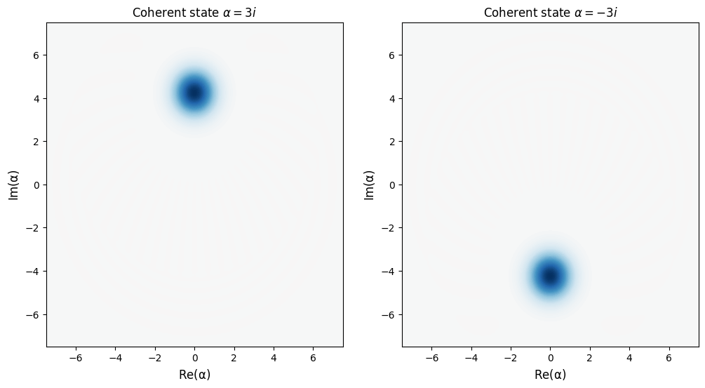
First: a reminder of what the Wigner function of two coherent states at \(x=0\) with opposite momentum look like:

Show code cell source Hide code cell source

N=30
rho1 = coherent_dm(N,3j)
rho2 = coherent_dm(N,-3j)

fig,ax = plt.subplots(1,2, figsize=(12,6))
plot_wigner(rho1, fig=fig, ax=ax[0])
ax[0].set_title(r"Coherent state $\alpha = 3i$")
plot_wigner(rho2, fig=fig, ax=ax[1])
ax[1].set_title(r"Coherent state $\alpha = -3i$")
plt.show()

Now, let’s compare a cat state and a mixed state.

Reminder

A cat state is a superposition of the wave functions:

\[ |{\rm cat}\rangle = \tfrac{1}{\sqrt{2}}|\alpha\rangle + \tfrac{1}{\sqrt{2}}|-\alpha\rangle \]

whereas a 50/50 “mixed” state is defined by the sum of the density matrices:

\[ \rho_{mix} = \tfrac{1}{2}\rho_\alpha + \tfrac{1}{2}\rho_{-\alpha} \]

Show code cell source Hide code cell source

N=30
rho1 = coherent_dm(N,3j)
rho2 = coherent_dm(N,-3j)
mixed = rho1 + rho2

psi1 = coherent(N,3j)
psi2 = coherent(N,-3j)
cat = psi1 + psi2

fig,ax = plt.subplots(1,2, figsize=(12,6))
plot_wigner(cat, fig=fig, ax=ax[0])
ax[0].set_title(r"Wigner function of a cat state of $\alpha$ and $-\alpha$")
plot_wigner(mixed, fig=fig, ax=ax[1])
ax[1].set_title(r"Wigner function of a mixed state of $\alpha$ and $-\alpha$")
plt.show()

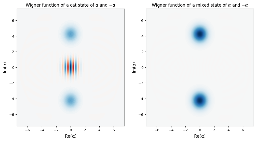
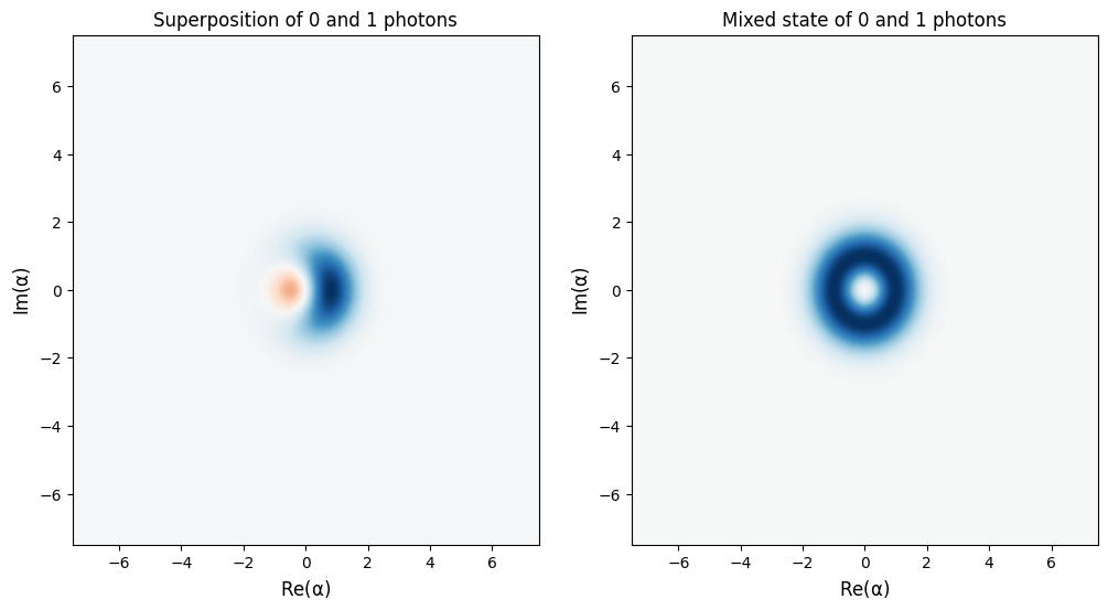
What is the difference? The “fringes” are gone! Similar to the coherences in the off-diagonal entries of the density matrix, the fringes of the cat state above are an indication of the “coherence” of the quantum superposition.

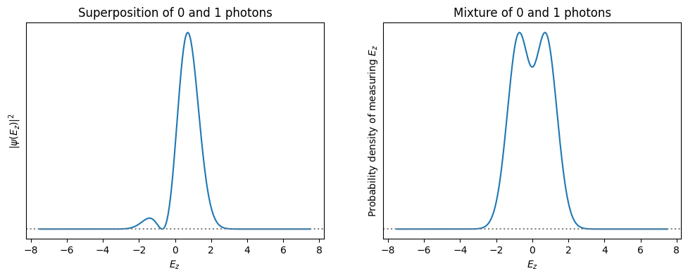
Without this “coherence”, the two “wave packets” do not interfere, as you can see if we plot \(|\psi(x)|^2\):

Show code cell source Hide code cell source

# A hack to calculate the probability distribution
x = np.linspace(-7.5,7.5,500)
wigner_mixed = wigner(mixed,x,x)
wigner_cat = wigner(cat,x,x)

prob_mixed = np.sum(wigner_mixed,axis=0)
prob_cat = np.sum(wigner_cat,axis=0)

# Now the plot
fig,ax = plt.subplots(1,2, figsize=(12,4))
ax[0].plot(x,prob_cat)
ax[0].set_title("Cat state")
ax[1].plot(x,prob_mixed)
ax[1].set_title("Mixed state")
ax[0].set_yticks([])
ax[1].set_yticks([])
ax[0].axhline(0,ls=':', c='grey')
ax[1].axhline(0,ls=':', c='grey')
ax[0].set_xlabel("$x$")
ax[1].set_xlabel("$x$")
ax[0].set_ylabel(r"$|\psi(x)|^2$")
ax[1].set_ylabel(r"$|\psi(x)|^2$")
plt.show()

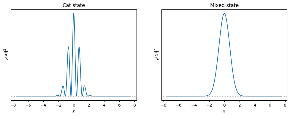
Of course, the proper interpretation of the lack of interference is, of course, that in the experiment there are not two wave-packets, but instead just one, and then we repeat the experiment over and over again, each time with only one coherent state of either \(\alpha\) or \(-\alpha\).

Example: Superposition vs. mixture of 0 and 1 photons

Show code cell source Hide code cell source

N=30
rho1 = fock_dm(N,0)
rho2 = fock_dm(N,1)
mixed = rho1 + rho2

psi1 = fock(N,0)
psi2 = fock(N,1)
sup = psi1 + psi2

fig,ax = plt.subplots(1,2, figsize=(12,6))
plot_wigner(sup, fig=fig, ax=ax[0])
ax[0].set_title("Superposition of 0 and 1 photons")
plot_wigner(mixed, fig=fig, ax=ax[1])
ax[1].set_title("Mixed state of 0 and 1 photons")
plt.show()

And now the “wave function” of the photon.

Reminder: What is the “wave function” of a photon?

A classical electromagnetic wave is a standing wave whose electric field oscillates in time: for example, for a given mode, we may have at a given fixed position in space an electric field with the following component in the z-direction:

\[ \vec{E}(t)\cdot \hat{z} = E_z(t) = E_0 \cos(\omega t) \]

where \(\hat{z}\) is a unit vector in the \(z\) direction. Note the similarity to the mass-on-a-spring, which oscillates in position:

\[ x(t) = x_0 \cos(\omega t) \]

In the mass-spring harmonic oscillator, we have a momentum \(p(t)\) that oscillates out of phase with the position:

\[ p(t) = p_0 \sin(\omega t) \]

In electromagnetism, there is also a magnetic field that also oscillates out of phase with the electric field :

\[ B_y(t) = B_0 \sin(\omega t) \]

(Note that if the \(E_z\) above belongs to a wave propagating in the \(x\) direction, then the magnetic field points in the \(y\) direction…)

The mapping from the mass-spring harmonic oscillator to the photon harmonic oscillator in this case is then:

• position \(\rightarrow\) electric field

• momentum \(\rightarrow\) magnetic field

Using this logic, for a photon, one can interpret the axes of the Wigner plots above as:

• Real part of \(\alpha\) \(\rightarrow\) \(E_z\)

• Imaginary part of \(\alpha\) \(\rightarrow\) \(B_y\)

The probability distributions of position \(|\psi(x)|^2\) and momentum \(|\phi(p)|^2\) are then replaced with probability distributions of \(E_z\) and \(B_y\):

• \(|\psi(x)|^2 \rightarrow |\psi(E_z)|^2\)

• \(|\phi(p)|^2 \rightarrow |\phi(B_y)|^2\)

Show code cell source Hide code cell source

# A hack to calculate the probability distribution
x = np.linspace(-7.5,7.5,500)
wigner_mixed = wigner(mixed,x,x)
wigner_sup = wigner(sup,x,x)

prob_mixed = np.sum(wigner_mixed,axis=0)
prob_cat = np.sum(wigner_sup,axis=0)

# Now the plot
fig,ax = plt.subplots(1,2, figsize=(12,4))
ax[0].plot(x,prob_cat)
ax[0].set_ylabel(r"$|\psi(E_z)|^2$")
ax[0].set_title("Superposition of 0 and 1 photons")
ax[1].plot(x,prob_mixed)
ax[1].set_ylabel(r"Probability density of measuring $E_z$")
ax[1].set_title(r"Mixture of 0 and 1 photons")
ax[0].set_yticks([])
ax[1].set_yticks([])
ax[0].set_xlabel("$E_z$")
ax[1].set_xlabel("$E_z$")
ax[0].axhline(0,ls=':', c='grey')
ax[1].axhline(0,ls=':', c='grey')
plt.show()

Demonstration: Thermal state of a harmonic oscillator (or a large spin)

Probability distributions for different temperatures:

Show code cell source Hide code cell source

N = 30
Ntemp  = 10
Npts = 100

Px = np.zeros([Npts,Ntemp])
T = np.linspace(0,5,Ntemp)

alpha_max = 7.5
x = np.linspace(-alpha_max,alpha_max,Npts)

fig, ax = plt.subplots()

line, = ax.plot(x, Px[:,0])

def update(i):
    wig = wigner(thermal_dm(N,T[i]),x,x)
    line.set_ydata(np.sum(wig,axis=0))

plt.ylabel("Probability density")
plt.xlabel("x")
plt.title("Thermal occupation from 0 to 5 quanta")
plt.ylim(-0.25, 4)  # Set the y-axis limits

anim = animation.FuncAnimation(fig, update, frames=Ntemp)
plt.close(fig)

HTML(anim.to_jshtml())

Once Loop Reflect